Titiler widget
As specified on the Tile layers features section, the Geobrowser can show on the map all the features exposing tiled services, such as WMS and Titiler. This section briefly describes the Titiler service and illustrates the geobrowser widget taking advantage of the TiTiler API.
Intro on Titiler
TiTiler, pronounced tee-tiler (ti is the diminutive version of the french petit which means small), is a lightweight application (FastAPI) focused on creating web map tiles dynamically from Cloud Optimized GeoTIFF, STAC or MosaicJSON.
Some Features:
- Cloud Optimized GeoTIFF support;
- SpatioTemporal Asset Catalog support;
- Virtual mosaic support (via MosaicJSON);
- Multiple projections (see TileMatrixSets) via morecantile;
- JPEG / JP2 / PNG / WEBP / GTIFF / NumpyTile output format support;
- OGC WMTS support;
- Automatic OpenAPI documentation (FastAPI builtin);
- Example of AWS Lambda / ECS deployment (via CDK).
For more info, see: https://devseed.com/titiler
Titiler layer and Geobrowser
On the Geobrowser, a feature exposing a Titiler tiled layer is represented on the results panel with the "Earth icon". If visible the layer is displayed on the map like any raster layer.
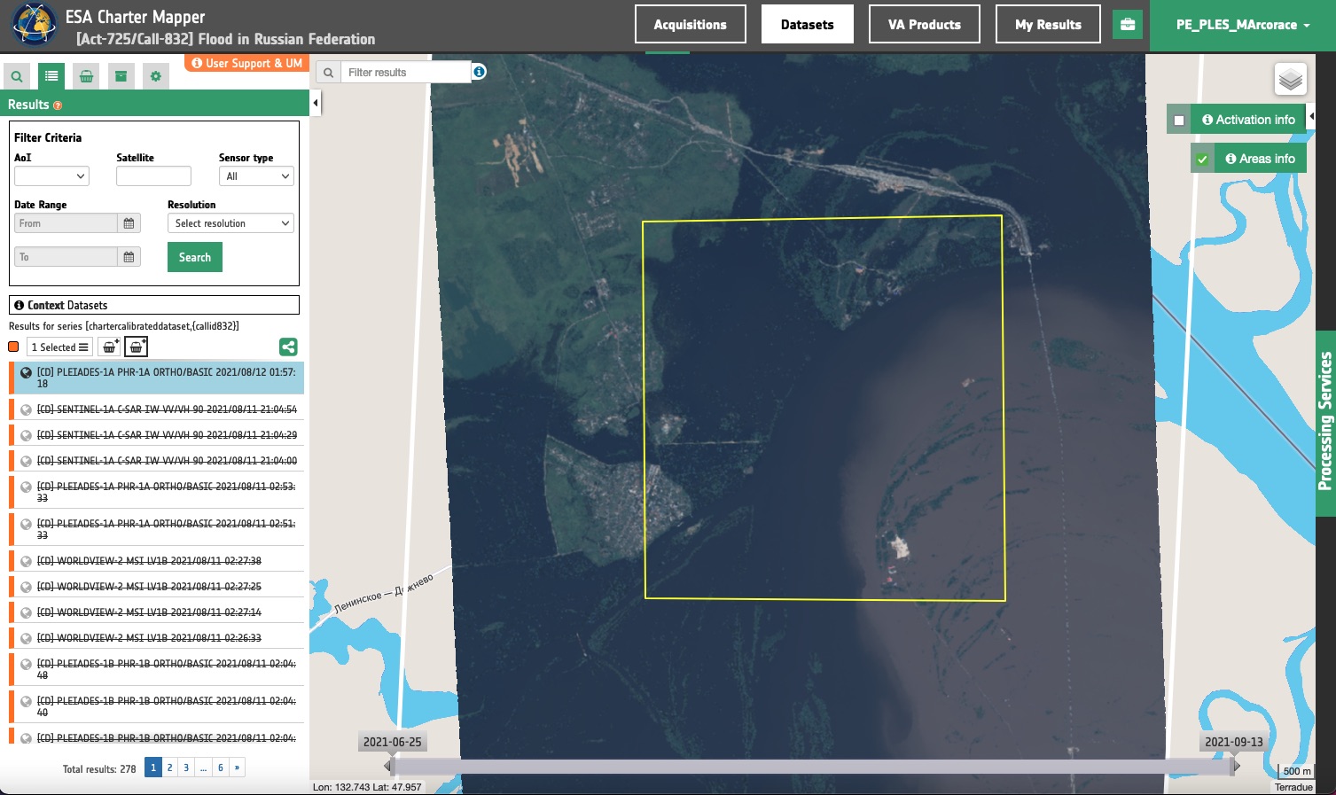
Opening the feature details panel, an additional widget called "Titiler options" is shown in the feature's details, inside the collapsible section "Layer styling".
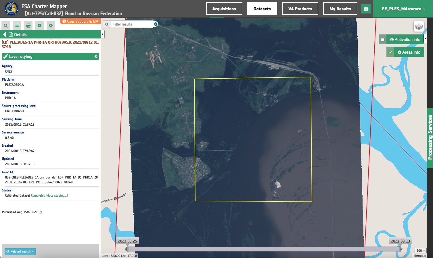
From this widget users can manipulate the TiTiler API options to see the layer in different ways and styles. More precisely, users can:
- choose one asset or select an assets combination;
- set and expression or select a predefinite color map (for one asset)
- set the histogram min and max value;
- apply a formula for color representation;
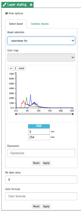
By clicking on the "Apply" button all the options will be applied, and the layer will be directly updated on the map, storing the options for the current session.
STAC and assets concept
The visualization and the options of a Titiler layer is based on the concept of Asset, defined on the STAC specification. The SpatioTemporal Asset Catalog (STAC) specification provides a common language to describe a range of geospatial information, so it can more easily be indexed and discovered. A 'spatiotemporal asset' is any file that represents information about the earth captured in a certain space and time.
For more info, see: https://stacspec.org/.
Any feature containing a TiTiler data has a set of assets (imagery, SAR, overviews, electro-optical reflectances, spectral indexes and so on); users can choose a single asset to view on the map, or a band-combination of three assets, mapped on the three RGB channel (Red, Green, Blue).
Single asset options
The single asset tab allows users to select one asset from the feature's available assets. If the asset is represented by a mono-band source, by default a grayscale image will be plotted.
There are 2 options: Color map, and Expression.
Color map
From the dropdown menu the user can select the color map from a predefined set. Color maps can be defined only for single band assets.
Expression
With this TiTiler option the user can employ a mathematical expression to combine one or multiple single band assets in one. For example, if a Dataset includes the red, green, blue, and nir single band assets the user can insert an expression like (nir-red)/(nir+red) to show in the map a virtual NDVI single band asset generated on the fly with this expression. Find more info about this advanced visualization functionality here.
Assets combination options
The assets combination tab allows users to select three assets for the three RGB bands and combine them. This tab doesn't have any option.
General options
Other useful options, common for both single asset or assets combination, are histogram min/max and color formula.
Histogram min/max
These two numerical inputs are used to define a range of minimum and maximum values of the digital number of the asset selected.
In the Charter Mapper there are several types of assets, each of them has a predefinite corresponding scale, as described in Table 1.
| type | description | Unit | Bit depth | Scaling factor | Valid Range |
|---|---|---|---|---|---|
| overview | RGBA color composite | Unitless | Uint8 | 1 | [0,255] |
| reflectance | TOA or BOA reflectance for VIS, RE and SWIR CBNs (e.g. blue, nir) | Unitless | Uint16 | 0.0001 | [0,10000] |
| brightness temperature | TOA or BOA brightness temperature for LWIR CBNs (e.g lwir11) | K | Uint16 | 0.01 | |
| spectral index | Spectral index as normalized difference of multiple CBN (e.g. NDVI) | Unitless | Float32 | 1 | [-1,1] |
| sigma nought | Sigma nought for L-, C-, X-band SAR data in each polarization (e.g. sigma0-HH-db) | dB | Float32 | 1 |
Table 1 - Description, Unit, Bit depth, Scaling factors, and valid ranges for the multiple types of assets available in the ESA Charter Mapper.
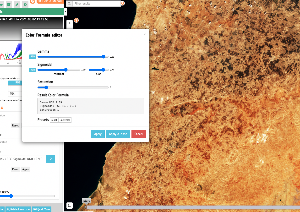
Color formula
With the color formula, it's possible to apply basic color-oriented image operations to the TiTiler image layer. The syntax is based on the rio-color plugin for the Cloud Optimized GeoTIFF in TiTiler and is the following:
Gamma RGB 1 Saturation 1 Sigmoidal RGB 3 0.5
where \(Gamma\), \(Saturation\) and \(Sigmoidal\) are the parameters described in Table 2.
| Color formula (rio-color color corrections) | ||||
| Correction | Parameter | Type | Description | Default values |
| Gamma | bands | string | Bands to which apply gamma correction. Use “RGB” for the three channels, “R” (or G, B) for single red-channel (or green-, blue-). | RGB |
| proportion | float | Gamma correction is a nonlinear operation that adjusts the image's channel values pixel-by-pixel according to a power-law. A value of gamma greater/lower than 1.0 lightens/darkens the image. proportion=0 results in a grayscale image, proportion=1 results in an identical image, proportion=2 is likely way too saturated. Reasonable gamma values range from 0.8 to 2.4. | 1 | |
| Sigmoidal | bands | string | Bands to which apply sigmoidal correction. Use “RGB” for the three channels, “R” (or G, B) for single red-channel (or green-, blue-). | RGB |
| contrast | integer | Enhances the intensity differences between the lighter and darker elements of the image. For example, contrast=0 is none, contrast=3 is typical and contrast=20 is a lot. | 3 | |
| bias | float [0,1] | Threshold level for the contrast function to center on (typically centered at 0.5). bias>0.5 darkens the image. | 0.5 | |
| Saturation | value | float | It applies saturation to an RGB array (in LCH color space). Multiply saturation by proportion in LCH color space to adjust the intensity of color in the image. As saturation increases, colors appear more "pure." As saturation decreases, colors appear more "washed-out." | 1 |
Table 2 - Default values for Color Formulas used for the generation of browse images in the PE (Credits: Rio-Color in GitHub). Such parameters are the ones available in the Rio Color color formula expression for COG in TiTiler.
The Color Formula field can be defined with a free text input. Alternatively, by clicking on the set color formula button users can populate the string with the help of a small interface.
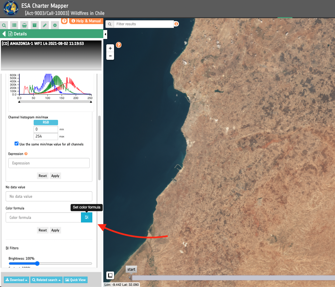
-
To switch from RGB to single channel settings (for Gamma and Sigmoidal) click on the RGB label (a chain-broken icon will appear on the label when mouseover);
-
To return to RGB selection (for Gamma and Sigmoidal) simply click on any channel label (a chain icon will appear on the label when mouseover);
-
The dialog is draggable and without backdrop so users can see the map result while setting the color formula sliders;
-
Both Apply and Apply and close buttons will apply the color formula to the TiTiler asset, but the second closes the dialog too;
-
Two presets are added (we can have more in the future): "reset", which remove any color formula effect, and "universal", which is the Universal color formula defined here. The presets will only set the values without directly applying the color formula (for further editing).
For more information, see https://github.com/mapbox/rio-color.
Histogram visualization
A feature exposing a TiTiler tiled layer can include a detailed histogram information for each asset, if available. The histogram provides the distribution of the pixel values. The space of pixel values is splitted in 256 buckets, and for each bucket is calculated the number of pixels inside of it.
With these data is possible to plot an histogram, allowing the user to:
- See the distribution of pixel values;
- Get the exact amount of pixel inside a bucket range;
- Set the histogram min/max value directly from a histogram interaction;
- Perform an vertical cut (by considering only the 99% of buckets in ascending order) to better show the histogram with a vertical stretch;
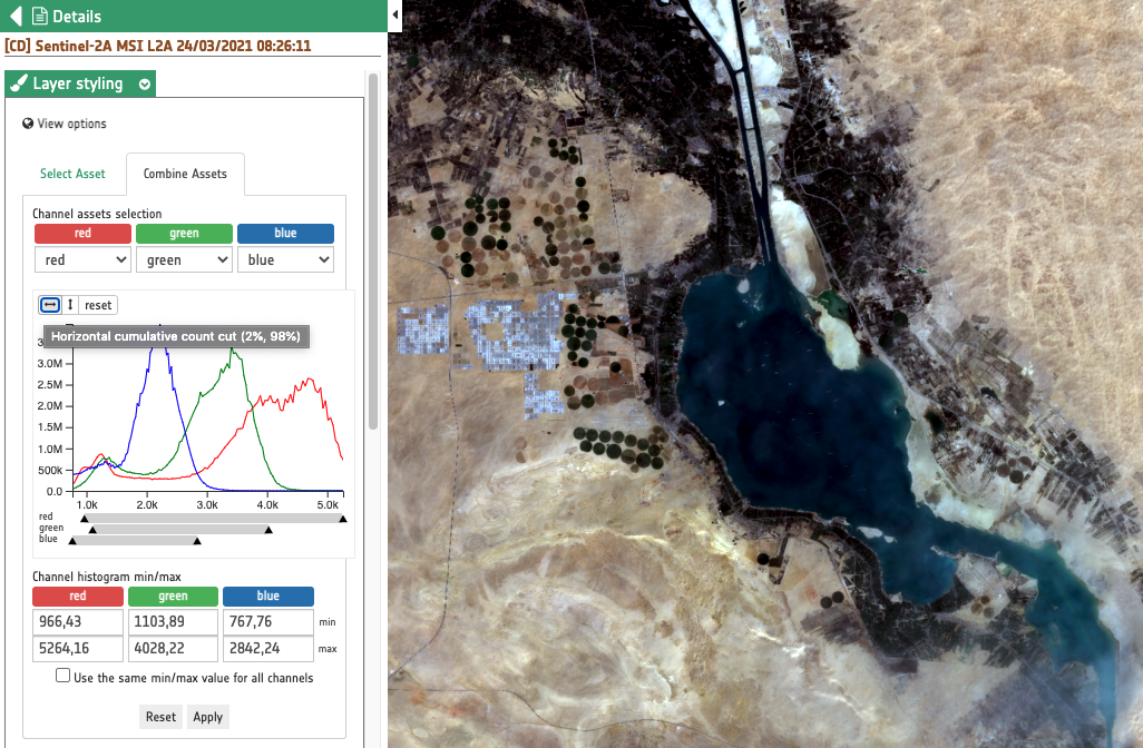
- Perform an horizontal cumulative cut ([2%-98%] of distribution), by a visual stretching of the histogram and by setting the right histogram min/max values.
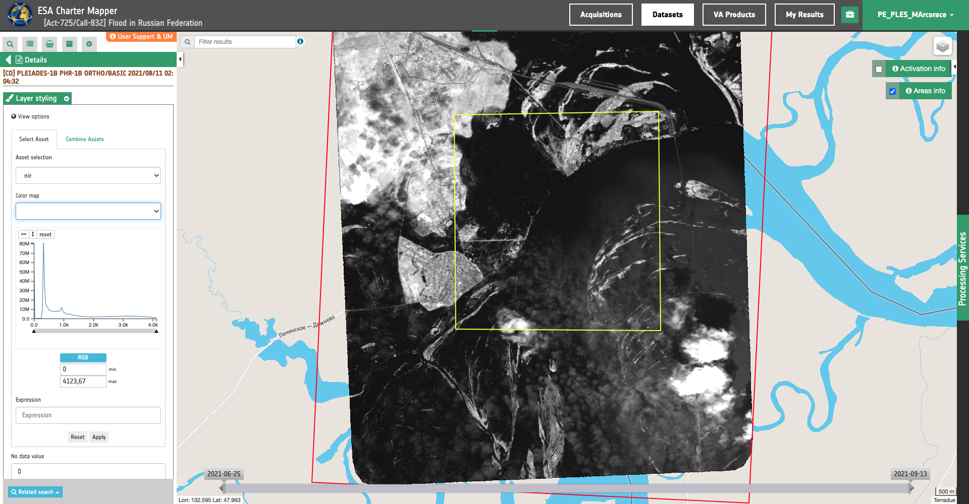
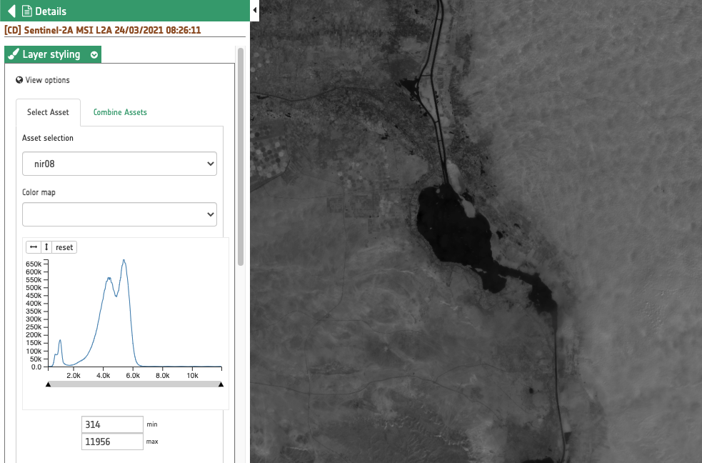
If a single band asset is selected, only one histogram function is plotted.
In this example an histogram is shown for the nir08 asset (single asset with single band):
By hovering the mouse on the graph it's possible to check out the amount of pixel for each pixel value range, as shown on this example:
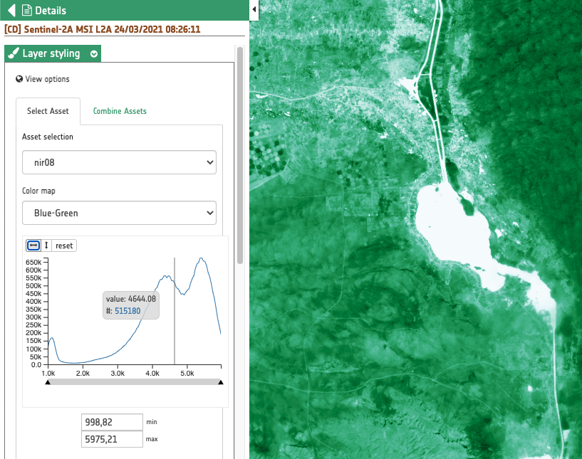
By dragging the range slider on the bottom of the graph it's possible to visually change histogram min/max values (it's always possible to manually change them from the min/max input fields):
Notice that when the histogram min/max is changed on the sliders, the changes are directly performed and the layer automatically updated, whereas users must click on the apply button if the min/max values are changed from the input fields.
Note
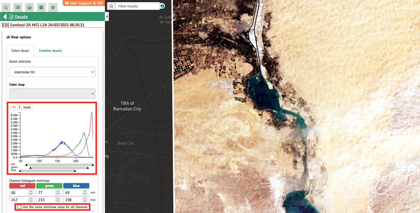
Notice that to enable changing min and max values in each RGB channel of an overview the option "Use the same min/max value for all channels" shall not be checked.
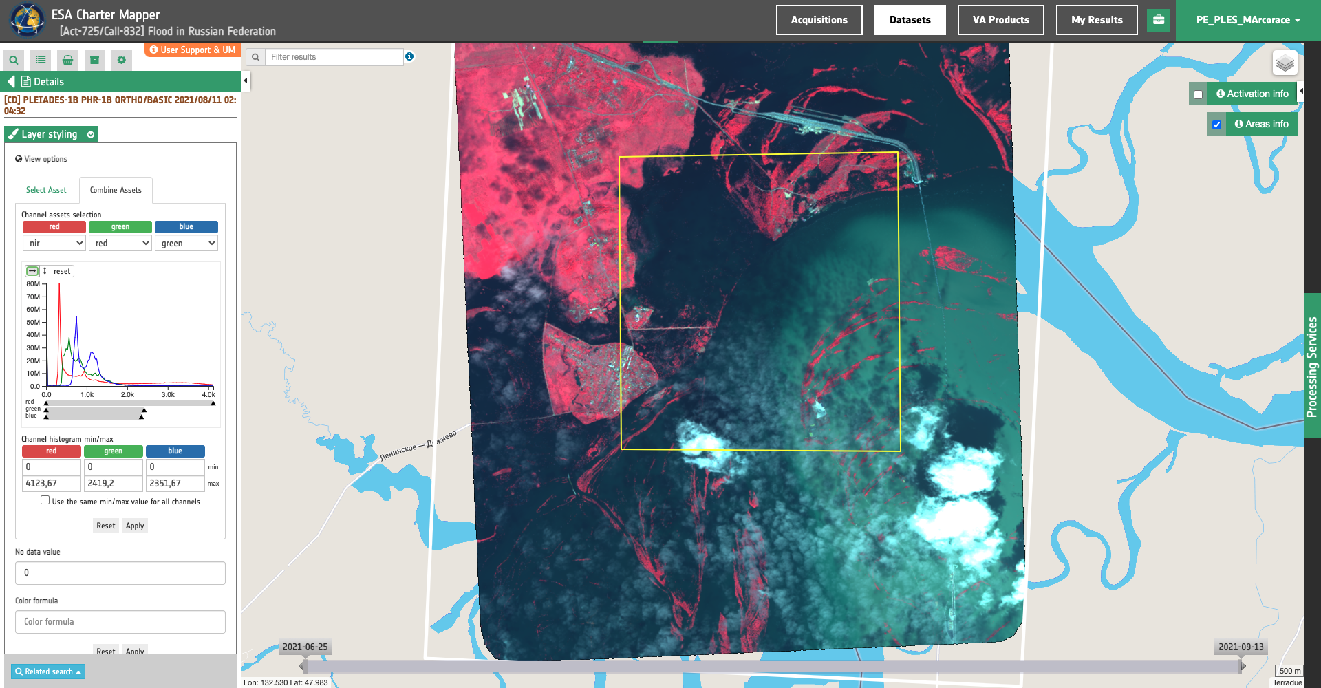
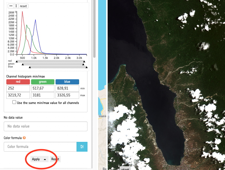
For multiple assets (or single asset with multiple bands) there are 3 histogram functions plotted, for the three RGB channels. Users can see the values for each bucket range and for each asset/band.
In this image there is an example of plotting multiple RGB assets histogram.
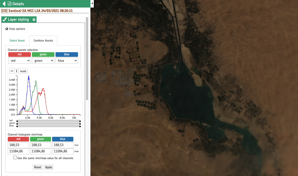
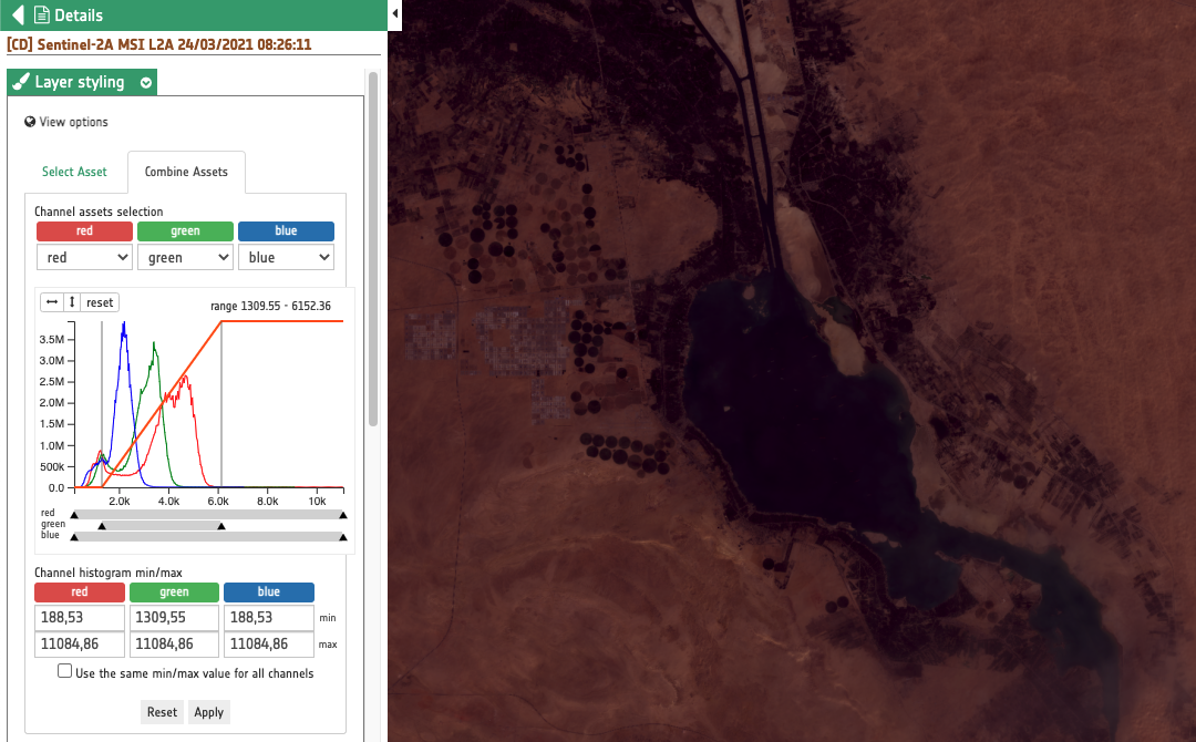
For multiple assets is also possible to separately set the histogram min/max, for each asset. The histogram min/max can be set by visual dragging of the sliders or by manual editing min/max input fields:
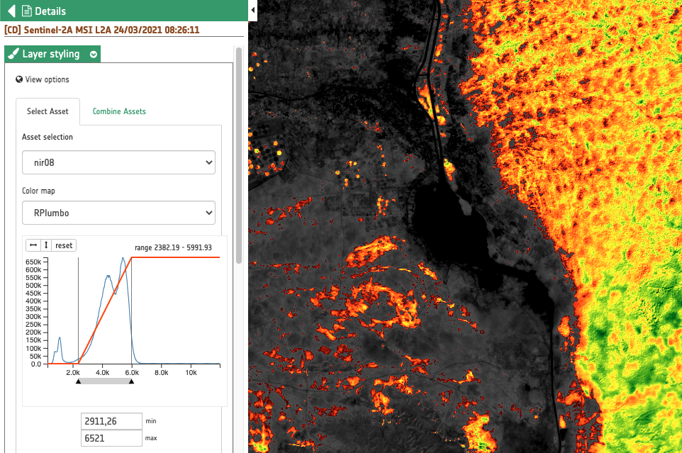
As shown above, full color ranges could not be optimized for a better layer visualization. It's possible to perform an auto select of the min/max value by a 2%-98% cumulative count cut, by clicking on the relative button:
The same applies for the vertical stretching:
The reset button resets the graph view.
Note
Notice that for multiple asset the histogram is plotted only if all three channels are selected.
Apply the same visualization settings to group of datasets
This function offers the possibility to apply the visualization settings defined for a Dataset to multiple Datasets. It aims to facilitate the visualization and fruition of multiple calibrated datasets and is available through the layer styling panel of a feature Dataset.
In the layer styling panel users can set different visualisation parameters (TiTiler options) for a feature dataset:
-
assets- the asset specified under Asset selection, -
rescale- the min and max values defined under Channel histogram min/max, -
asset_as_band- the assets specified under red green and blue channel under Combine Assets, -
colormap_name- the key specified under Color Map, -
expression- the expression, as an example(nir-red)/(nir+red), specified under Expression, -
resampling_method- the resampling method specified under the Options tab from the left panel of the interface (averageis the default), -
nodata- the no data value, as an example0, specified under No Data value.
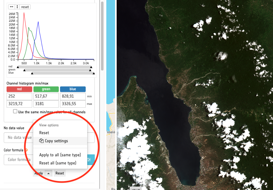
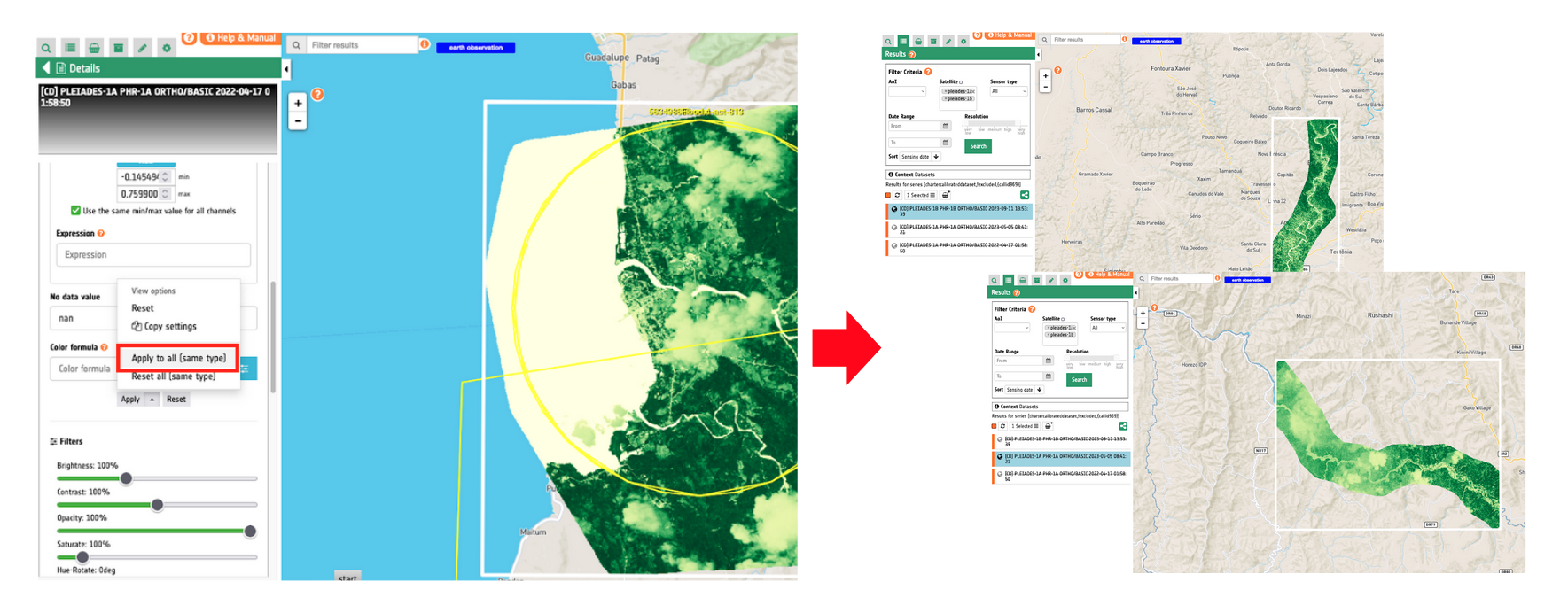
From the layer styling panel users have then the possibility to apply these settings to the selected dataset only or to all the datasets of the same type. Users can also copy the setting of one dataset and paste them to another one (similar to a “copy layer style” functionality available in GIS software). From the panel this functionality is offered as an extension of the Apply button.
By opening the Apply button caret a dropdown menu will appear offering the following options:
-
Reset- to reset the layer styling of the current dataset, -
Copy settings- to copy the current layer style to the clipboard, -
Paste (apply)to paste the layer style to the current feature dataset, -
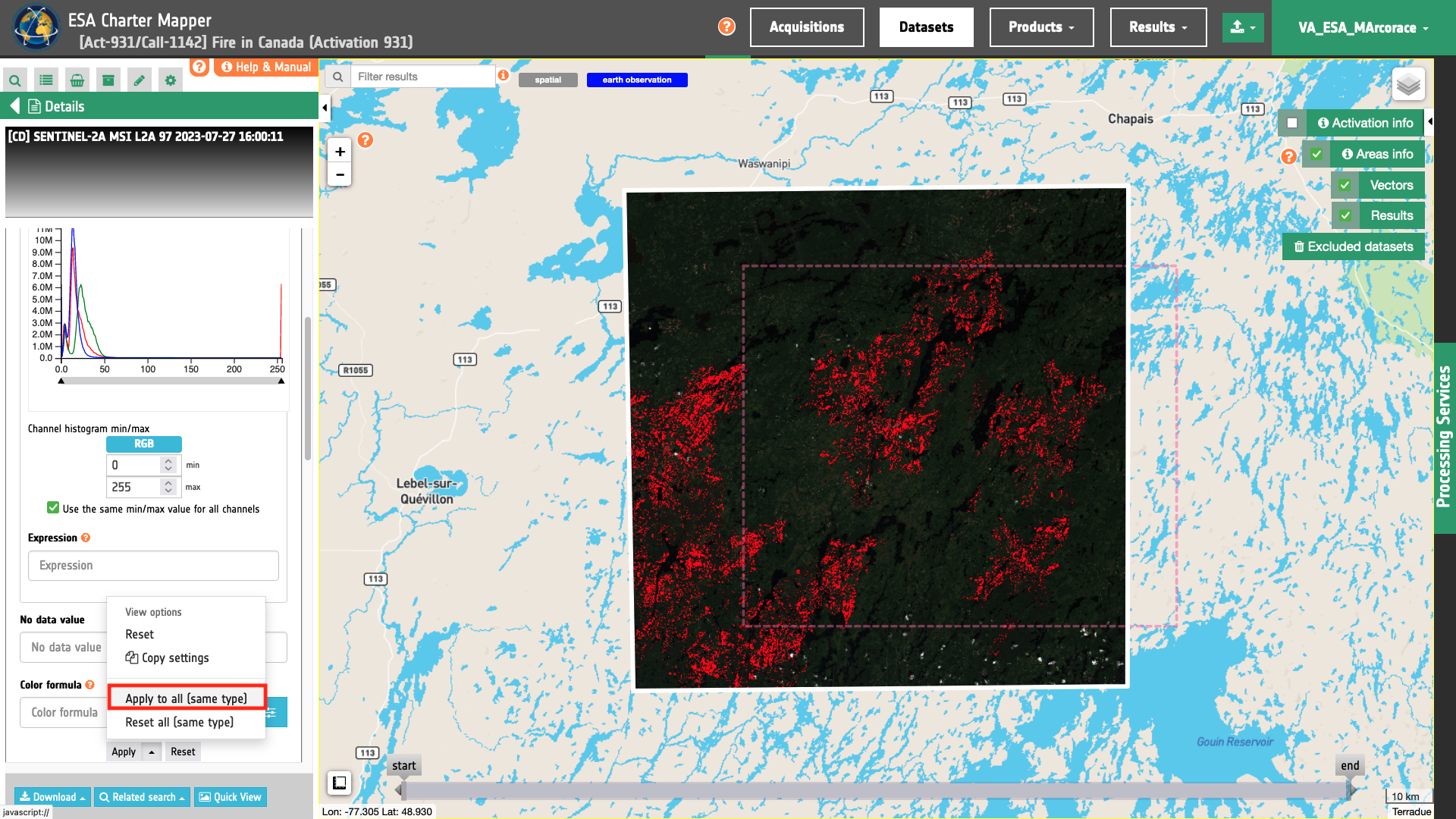
Apply to all (same type)to apply the layer styling to all datasets of the same type, -
Reset all (same type)- to reset the layer styling for all products of the same type (including the current product).
Warning
Datasets of the same type are the ones from the same EO mission (e.g. RCM) and having the same product type (e.g. GRD). This limit is in place because multiple visualization settings (e.g. assets, rescale, histogram min / max, etc.) are not applicable to heterogeneous datasets.
Note
The visualization settings are persisted at the browser user local storage.
Possible use cases for the above described functionality are described in the below sections.
Apply same visualization for overview assets
Typical use case is to switch for all the Datasets in the Results list from a default overview (e.g. overview-trc) to another one (e.g. overview-bav). In this way the user can easily change overviews of all datasets in the map without doing it manually one by one.
Apply same visualization for single band assets
Another example is the visualisation of multiple normalised difference single band assets with the same min max. Thanks to this functionality the user can apply the same expression to create a normalized difference on the fly (or select an index already present in the Dataset as the ndvi one) and have the same Min/Max to all the other single band assets shown in the map.
As an example from the Filter Criteria box filter EO data by setting under the Satellite filter pleiades-1a and pleiades-1b and then select a Pléiades calibrated Dataset. Access the Details of the selected feature and from the layer styling panel set the following:
-
Asset selection:
ndvi -
Color Map:
Yellow-Green -
Channel histogram min/max: min value as
0.3and max value as0.7 -
No data value:
nan
After clicking on the Apply to all (same type) button all the other Pleiades-1 datasets will show as default asset in the map the one with the same visualization options of the one just edited.
Apply same visualization for single band assets after binarization
When the user wants to apply on the fly the same image binarization to all features using TiTiler expressions. This is very useful to quickly estimate standing waters from the on the fly binarization of multiple Sigma nought single band assets using the same threshold.
Apply same visualization for customized RGB composites from single bands
Another common use case is the application of the same RGB combination and image stretching to all the other datasets using Combine Assets. The functionality takes the parameters of a Combine Assets made by the user for a selected dataset and it applies the same params to all the other datasets of the same type
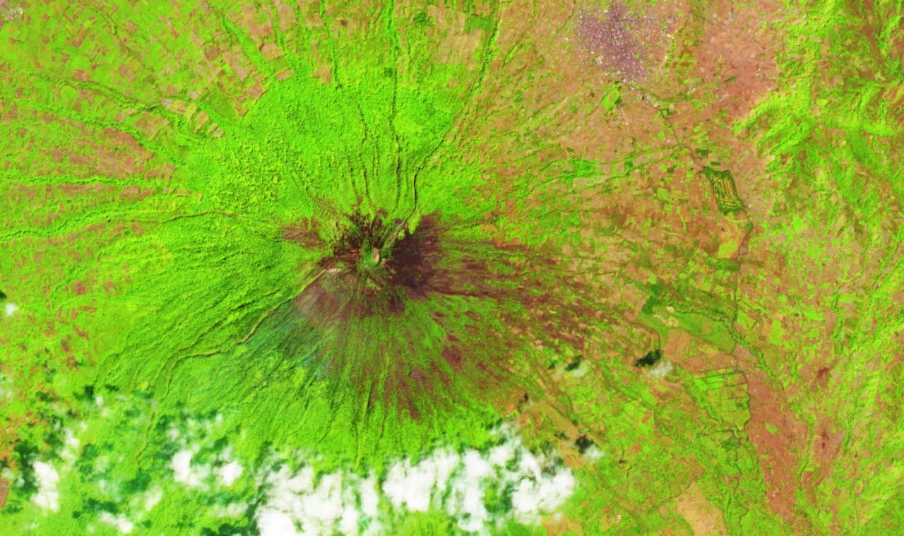
Quickview button to crop and export one or two images
For TiTiler layers it is possible to select an area of the layer on the map and download it as a cropped image. The crop export maintains all the current visualisation settings applied to the image e.g. through the asset selection, histogram, color map and so on. It exports the portion of the image exactly as it is shown on the map.
Export cropped image from a single feature
From the relative feature's Details panel on the left of the interface, users must click on the Quick View button to export a crop from a TiTiler layer.
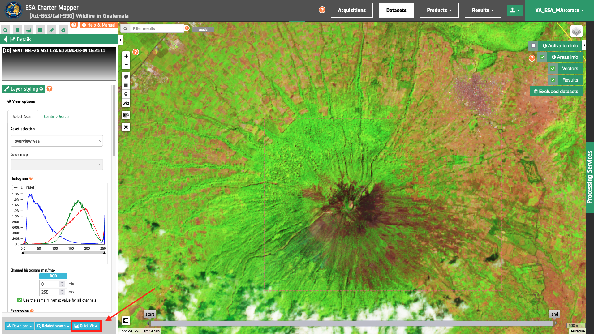
After clicking on the Quick View button a dedicated panel (little modal dialog) will be opened.
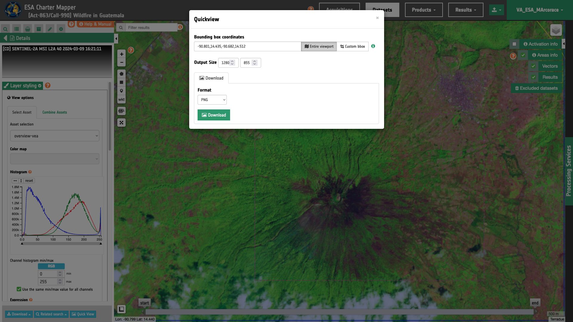
From this panel users shall specify the following 3 parameters which are necessary to export a portion of the TiTiler layer into an image:
-
Bounding box coordinates - either by manually inserting the coordinates or by deriving them automatically with the
Entire viewportor theCustom bboxbuttons. -
Output size - by inserting size of pixels (rows and columns of the array) of the output image from a resampling of the TiTiler layer
-
Format - by selecting one among the PNG, GeoTIFF or JPEG formats.
Bounding box coordinates
By default the bounding box is the one of map extent. However, using this panel users can change it as needed. In the definition of the Bounding box coordinates, if the user clicks on the Custom bbox button can draw the bounding box directly in the map.
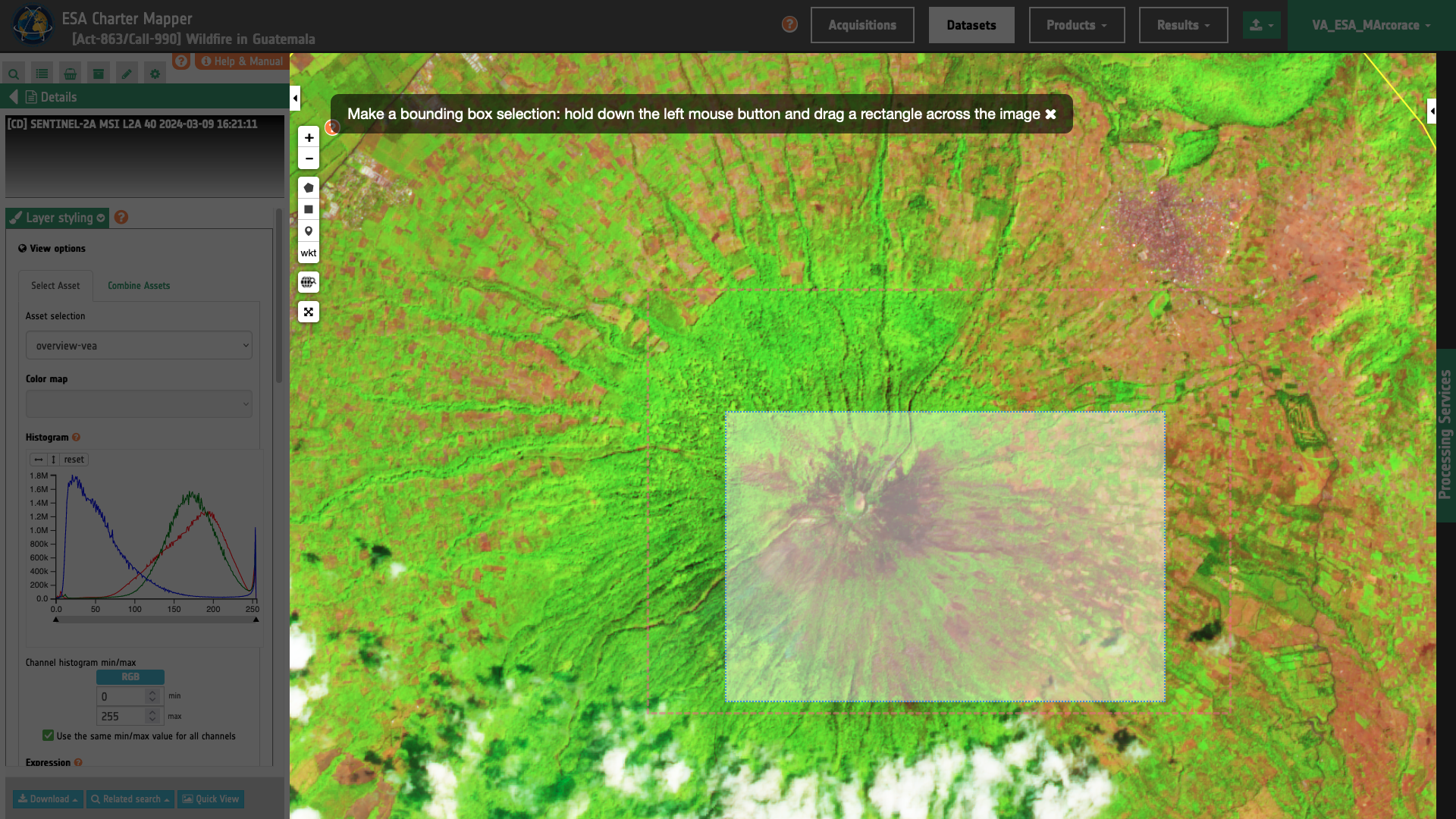
If needed, resulted coordinates from the drawn polygon can be then re-defined manually by adjusting the values to have a more precise crop area.
Output size
By default the output size of the image is set to 1280 x 759 pixels. However, output image size can be changed by the user as necessary. The crop export is limited in terms of resolution (max 2000 x 2000 pixels).
Format
To define the format of the output image just select one from the dropdown menu. Supported export formats are PNG, JPEG and GeoTIFF. The GeoTIFF format also contains spatial metadata, so it's possible to import the downloaded GeoTIFF directly on other GIS applications, like QGIS.
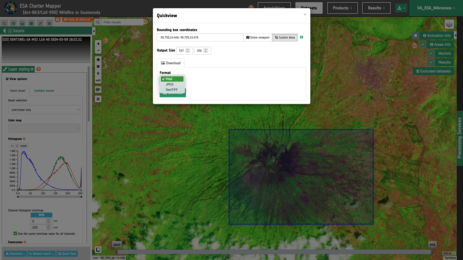
Download
By clicking on the Download button the image will be downloaded (or opened in a new window, depending on the browser and on the selected format).
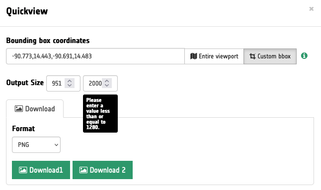
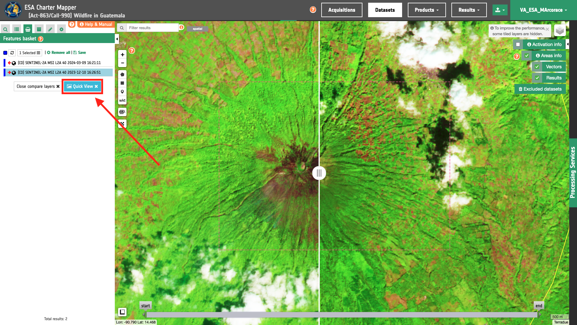
Export cropped images when comparing two layers
The QuickView functionality is also applicable when comparing two layers with the slider. In this case the Quick View button appears next to the Close Compare layers one.
As for a single feature, the QuickView panel provides the same options to define the bounding box for cropping the TiTiler layer as well as the size and format of the output image.
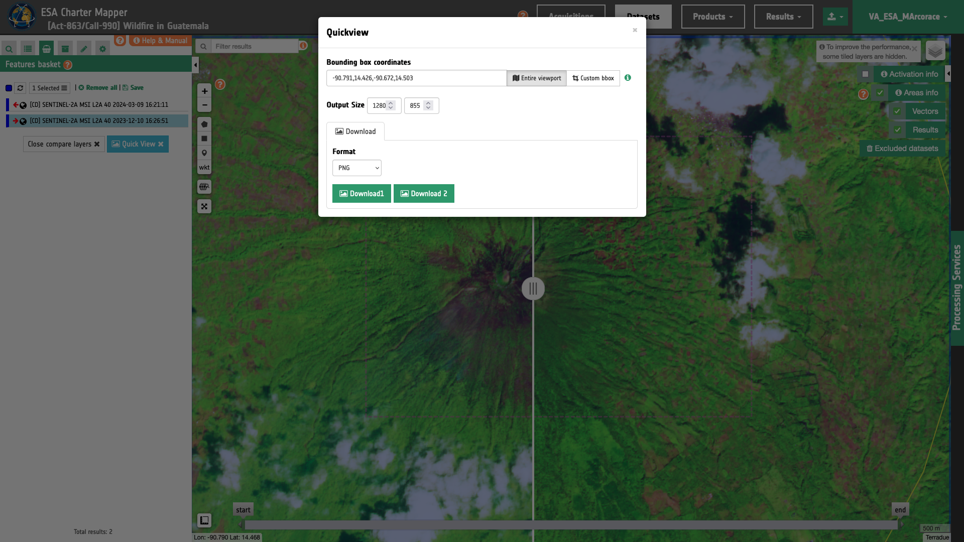
In addition to that, the Download1 and Download2 buttons allow the user to download the two images that the user is comparing with the slider.
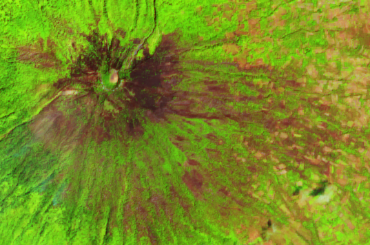
Before the event quick view image
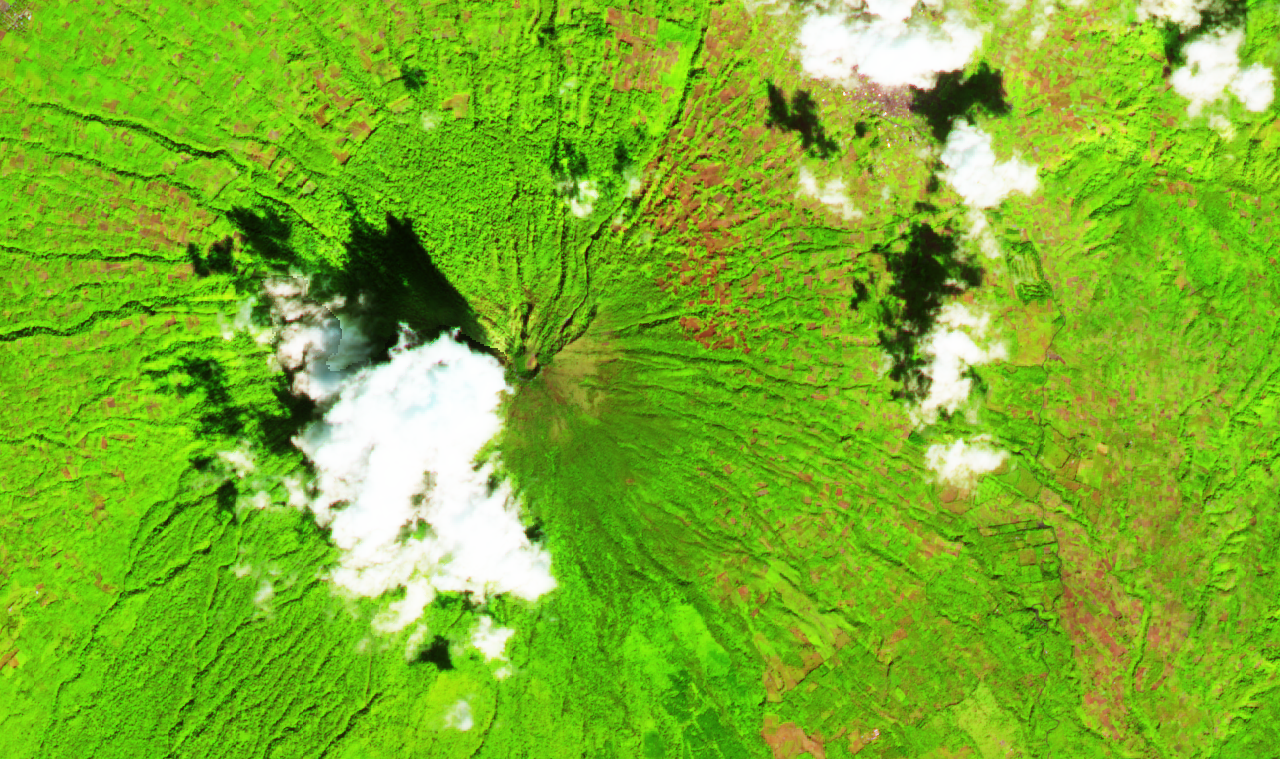
After the event quick view image