Visual comparison of EO data and Products

Compare pre and post event images

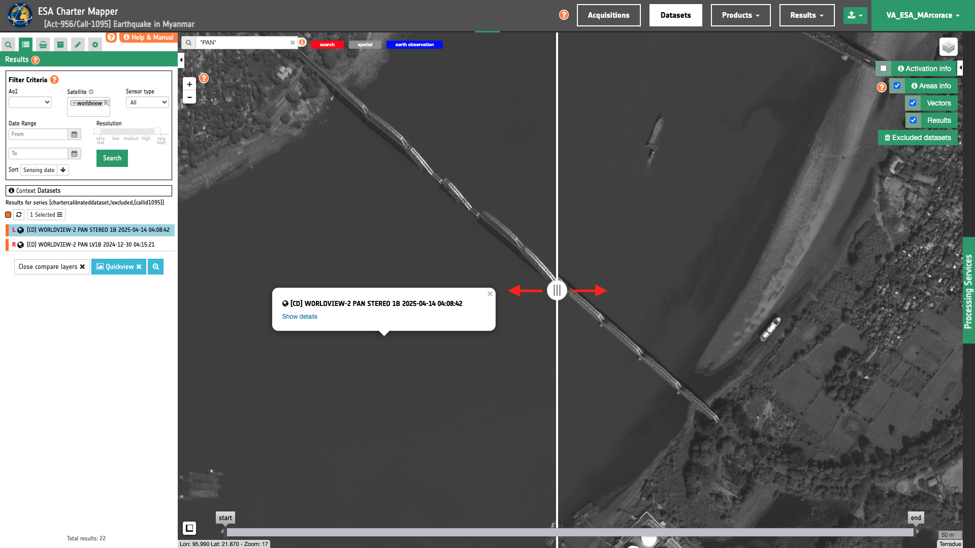
The ESA Charter Mapper offers multiple visualization tools. As an example, to enhance the visualization of multiple layers, the geobrowser also provides a Vertical Slider Bar to visually compare two images (e.g. pre- and post-event). This is possible by selecting from the Results panel two features (e.g. two Calibrated Datasets) having active tiled layers.

Note

A product with tiled layer active (e.g. when for a Dataset an overview is visible in the map) has the world icon . For more information please refer to the section of the user manual about the Geobrowser Layout.

To visually compare two Assets from 2 Datasets or Results from processing listed in the Results panel:

select a pair of features (e.g. 2 Calibrated Datasets),
click on the button located on top of the list,
from the drop-down list click on Compare Layers,

figure 1A

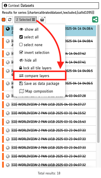
after that the two features will be both shown in the map divided by a vertical slider bar.

Figure 1 - Compare Layers function and visual comparison of the Innwa bridge in Sagaing, Mandalay, Myanmar before and after the 7.7-magnitude earthquake of 28 March 2025 using a pair of Worldview Panchromatic assets with the vertical slider bar in the ESA Charter Mapper (Image credit: Maxar, USGS).

More information about how to activate image comparison slider bar for a pair of Datasets can be found here.

Compare an asset with the basemap

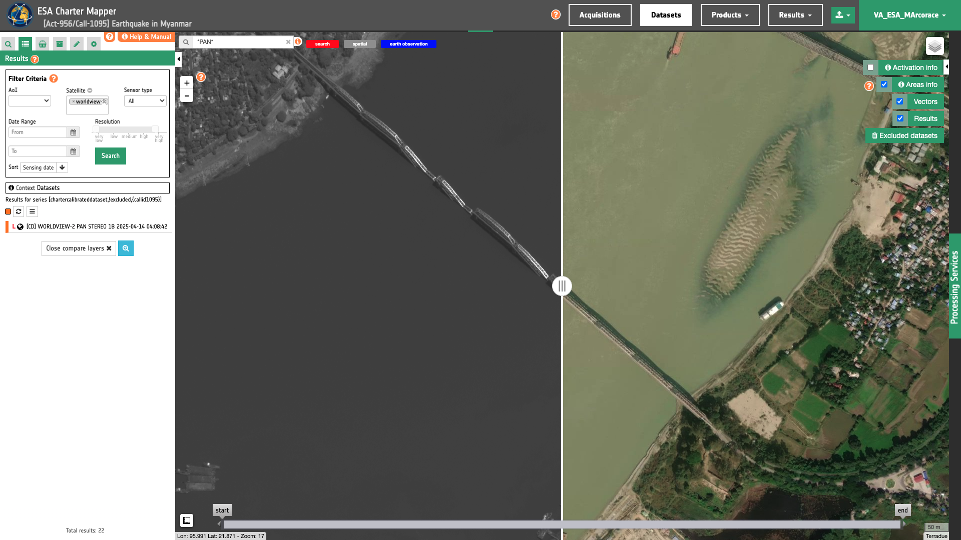
The Vertical Slider Bar can be also employed to compare a crisis image with a baselayer (e.g. global satellite imagery layer).

To visually compare an asset from a dataset listed in the Results panel against the current baselayer (e.g. Satellite Imagery layer selected from the button located in the top right corner of the map):

select one feature (e.g. an optical Calibrated Dataset after the event),
click on the button located on top of the list,
from the drop-down list click on Compare Layer with base map,

figure 2A

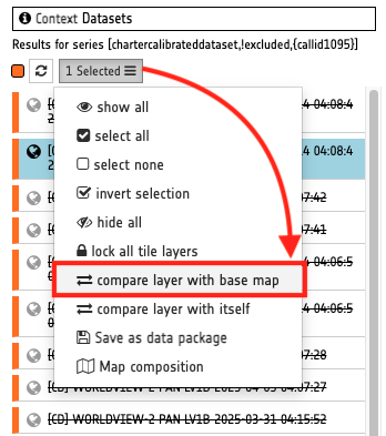
after that the crisis image and the basemap will be both shown in the map divided by a vertical slider bar.

Figure 2 - Compare Layers function and visual comparison of the Innwa bridge in Sagaing, Mandalay, Myanmar before and after the 7.7-magnitude earthquake of 28 March 2025 using a post-event Worldview Panchromatic asset and the Natural Earth base layer with the vertical slider bar in the ESA Charter Mapper (Image credit: Maxar, USGS).

Compare assets from the same dataset or result

When needed the user can also Vertical Slider Bar can be also employed to compare two intra-sensor assets from the same calibrated dataset (e.g. nir VS red) or two assets from the same Result of a service (e.g. the flood map against the post-event backscatter).

To visually compare two assets from a dataset listed in the Results panel:

select one feature (e.g. an optical Calibrated Dataset after the event),
click on the button located on top of the list,
from the drop-down list click on Compare Layer with itself,

figure 3A

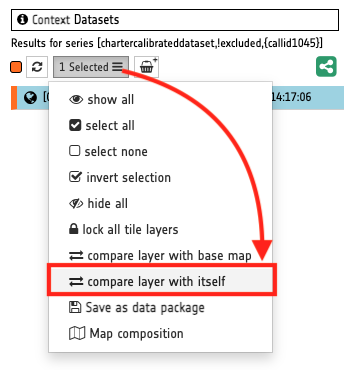
after that the selected feature and a copy of it will be shown in the map divided by a vertical slider bar.

The second dataset is a virtual copy of the selected one. In one dataset you can choose an asset (e.g. overview-trc) and in the second one another one you want to compare with (e.g. overview-civ).

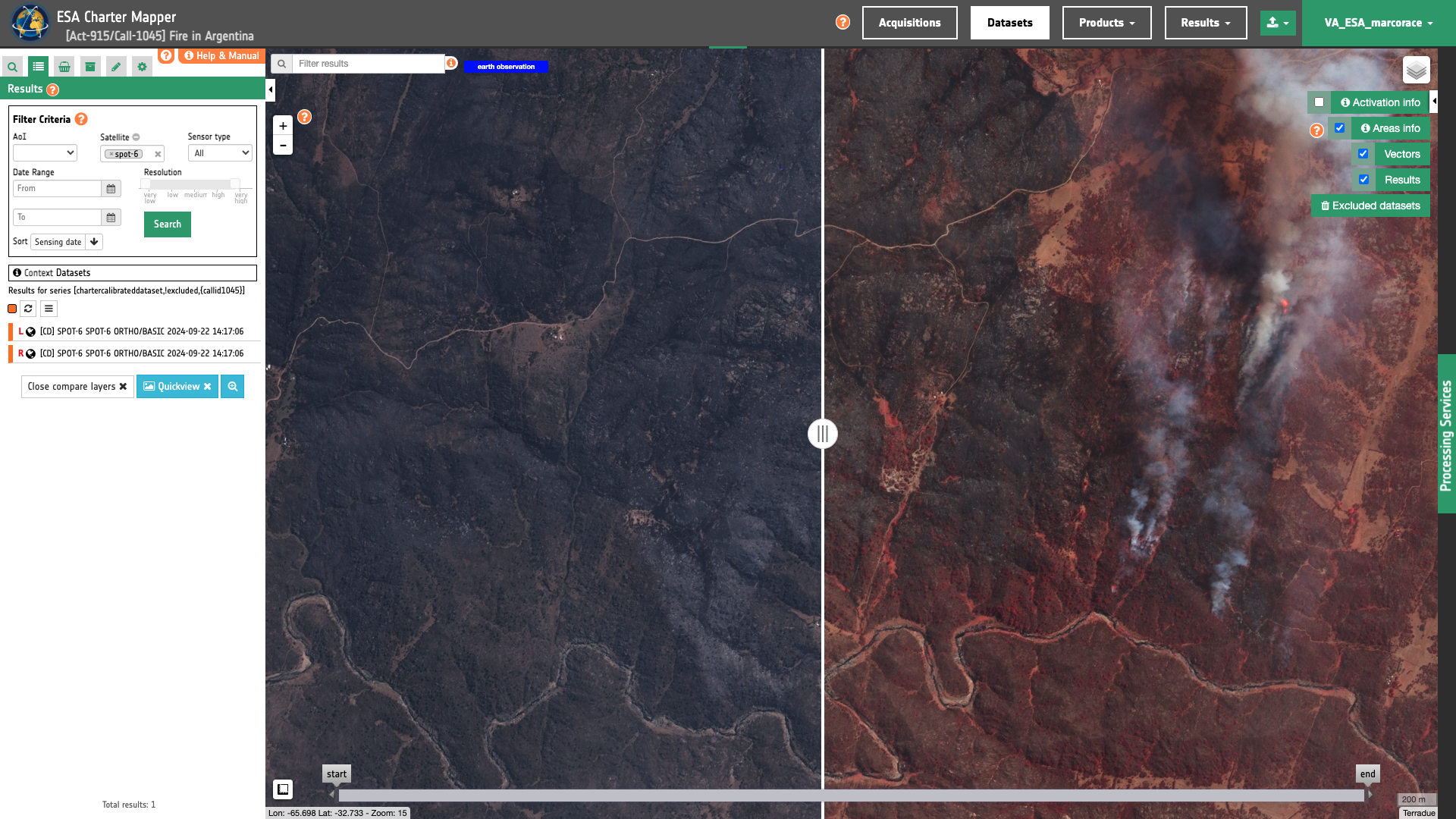
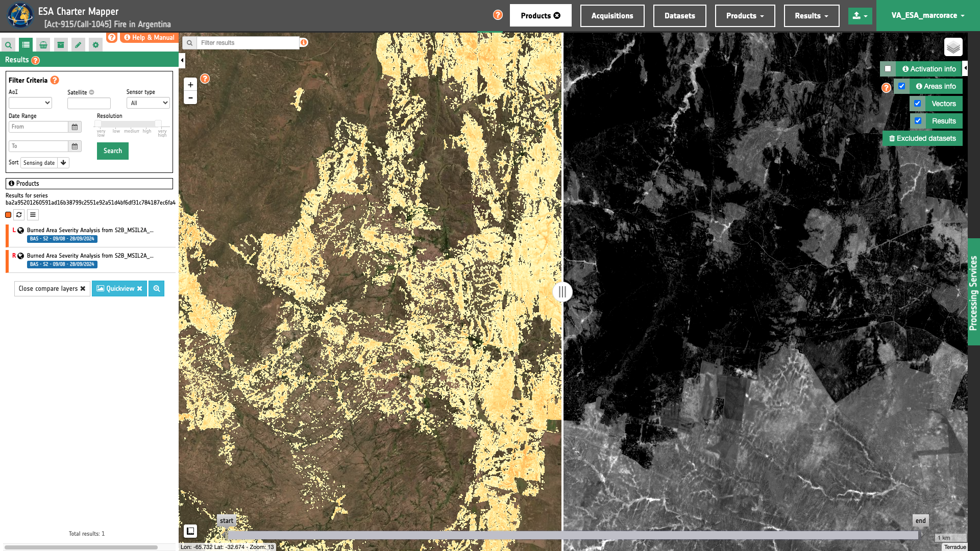
Figure 3 - Compare Layers function and visual comparison of burned area near San Luis, Argentina as of 22 September 2024 using a true color composite asset (left) and a color infrared false color composite asset (right) retrieved from the same SPOT-6 calibrated dataset with the vertical slider bar in the ESA Charter Mapper (Image credit: Airbus, CNES).

In the same manner it is also possible to compare assets from a Result of a processing service. The below figure shows an example of how to compare two assets from a result of the Burned Area Severity (BAS) service.

Figure 4 - Compare Layers function and visual comparison of burned area severity near San Luis, Argentina as of 22 September 2024 using the burned area severity overview asset (left) and the post-event NBR index asset (right) retrieved from the same BAS result with the vertical slider bar in the ESA Charter Mapper (Image credit: Copernicus, ESA).

Compare EO data and Products via the Features Basket

In the ESA Charter Mapper it is also possible to visually compare the results obtained from a processing service (e.g. the NDVI from the OPT-Index processor) with a single-band asset or an overview product (e.g. Color Infrared Vegetation RGB composite) from the calibrated EO data employed as input of the same processing service (e.g. Color Infrared Vegetation overview from TOA reflectance).

In order to compare the Spectral Index with the original image, it is useful to have the product displayed over the satellite imagery. This can be done using the Features Basket function available in the ESA Charter Mapper. More information about the Features Basket function can be found here.

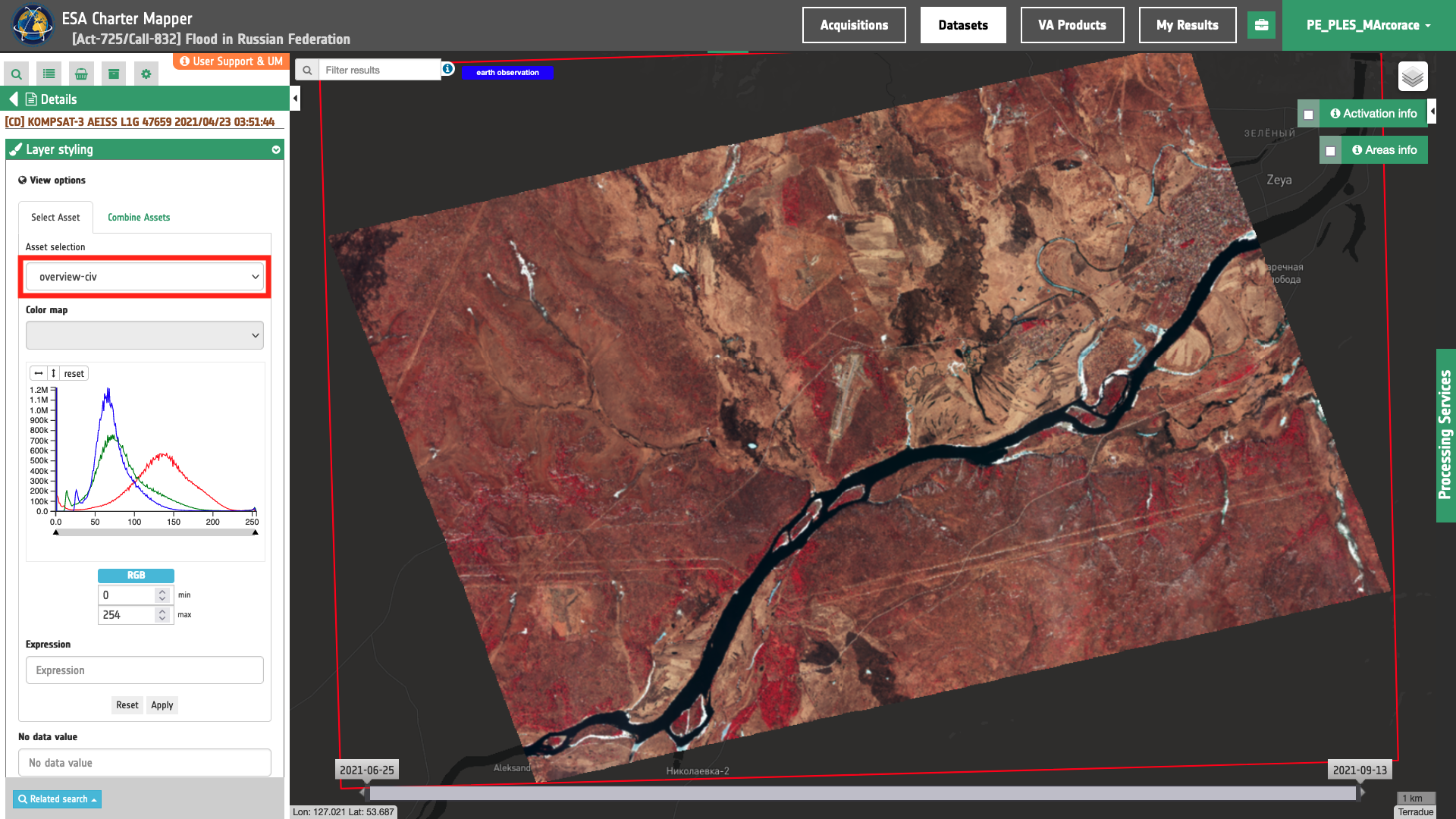
First step is the identification of a suitable EO data to be processed over an AOI, e.g. a Kompsat-3 multispectral Calibrated Dataset.

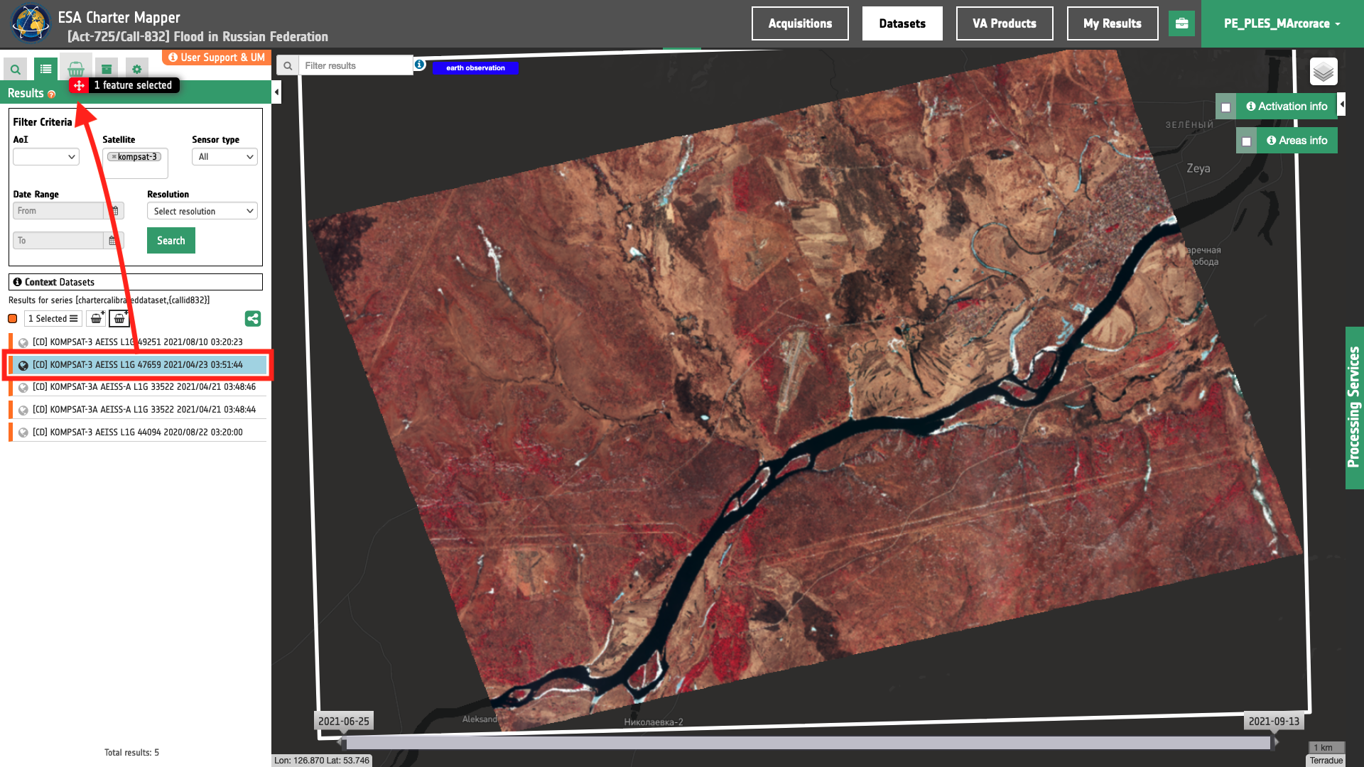
Figure 5 - Color Infrared Vegetation overview from Kompsat-3 data over the Russian Federation (Image credit: KARI).

Once the image of interest is identified, it is worth dragging and dropping from the Results tab the Dataset directly into the Features Basket. This preliminary step will facilitate the retrieval of the EO data in the following steps and will be a reference location for future use of the same Dataset.

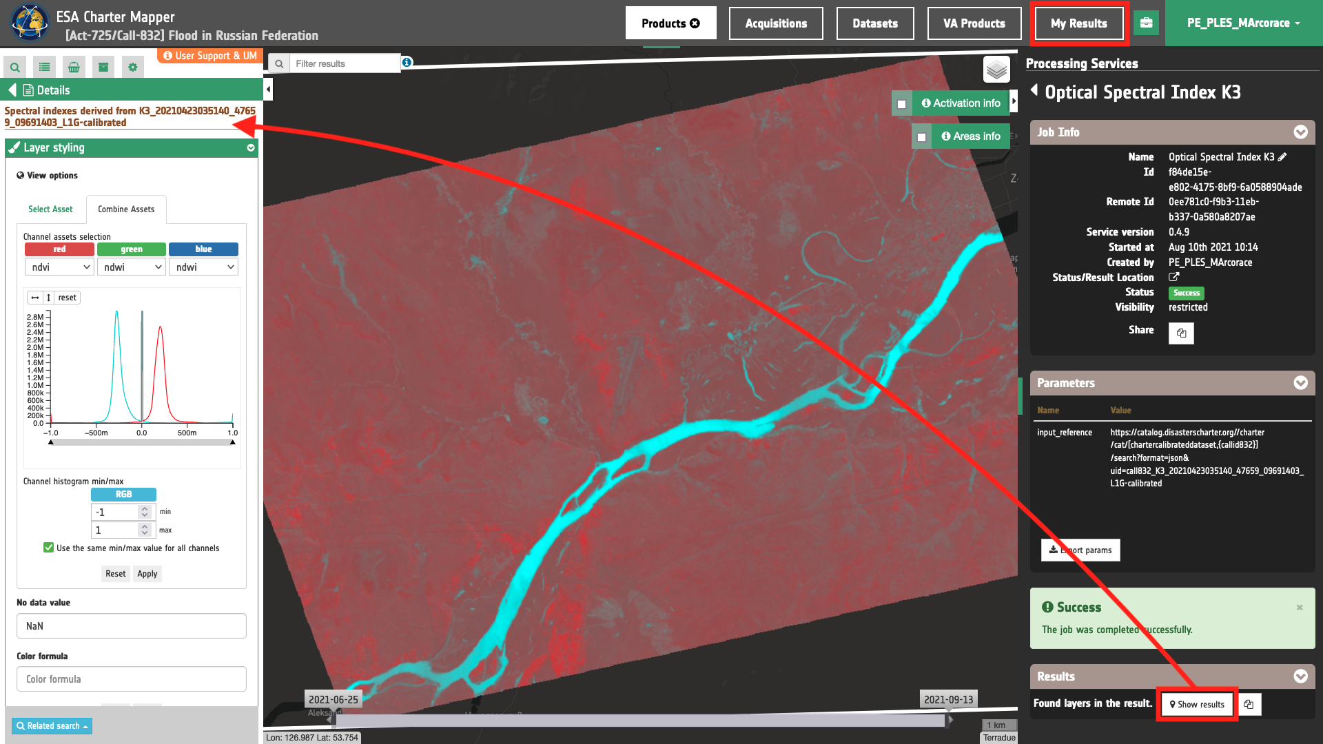
Figure 6 - The drag and drop of a Kompsat-3 Calibrated Dataset from the Results panel into the Feature basket (Image credit: KARI).

Later the OPT-Index processor can be executed by setting as input reference the same dataset included in the Feature Basket. More information about the Optical Spectral Index service function can be found by looking at the OPT-Index tutorial as well as the OPT-Index service specifications. Once the job is succeeded the Result will be accessible under the Result panel in the left by clicking on the My Results button in the Data Context Menu or by clicking on Show results under the Processing Result tab in the right panel of the interface.

Figure 7 - Red-Cyan RGB composite from NDVI (Red) and NDWI (Cyan) indexes derived from Kompsat-3 data over the Russian Federation (Image credit: KARI).

The Result of the OPT-Index can be also included into the Feature Basket where the source calibrated Dataset is stored. To do so simply drag and drop the layer under Products from the Results tab into the Feature Basket.

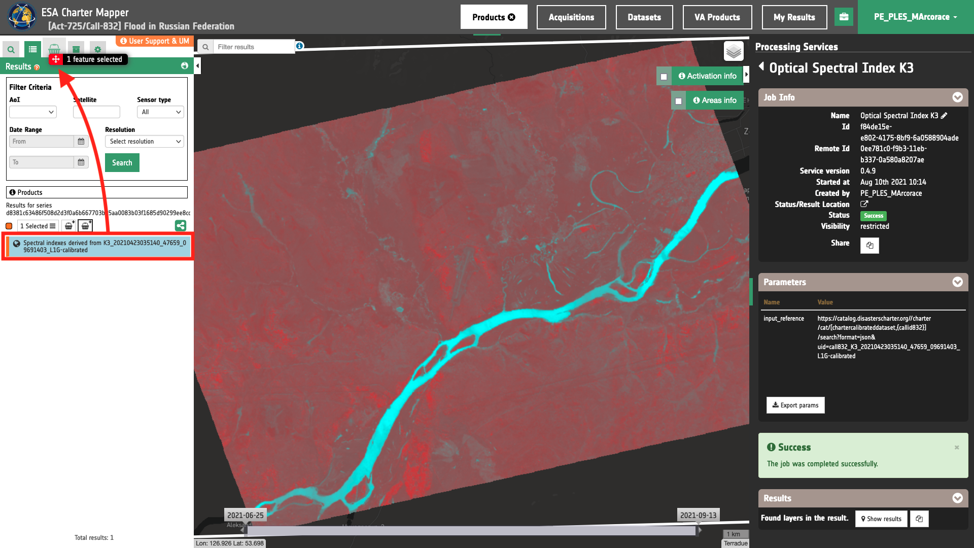
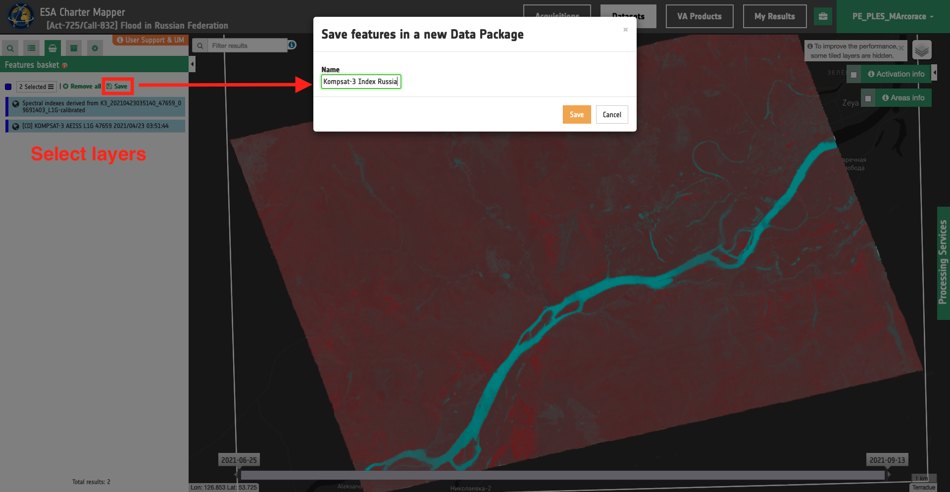
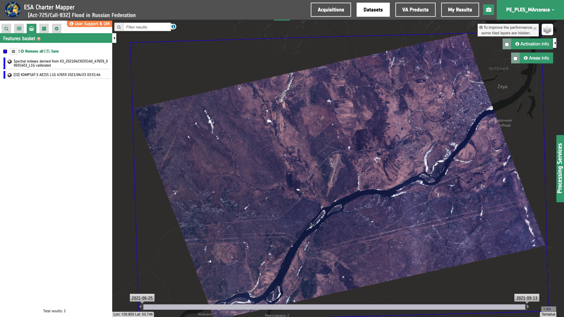
Figure 8 - The drag and drop of a Spectral Index Product derived from a Kompsat-3 Calibrated Dataset from the Results panel into the Feature basket (Image credit: KARI).

After that by opening the Feature Basket only the two Products (Calibrated Dataset and Spectral Index Product) contained in the basket will appear in the map as shown in Figure 9.

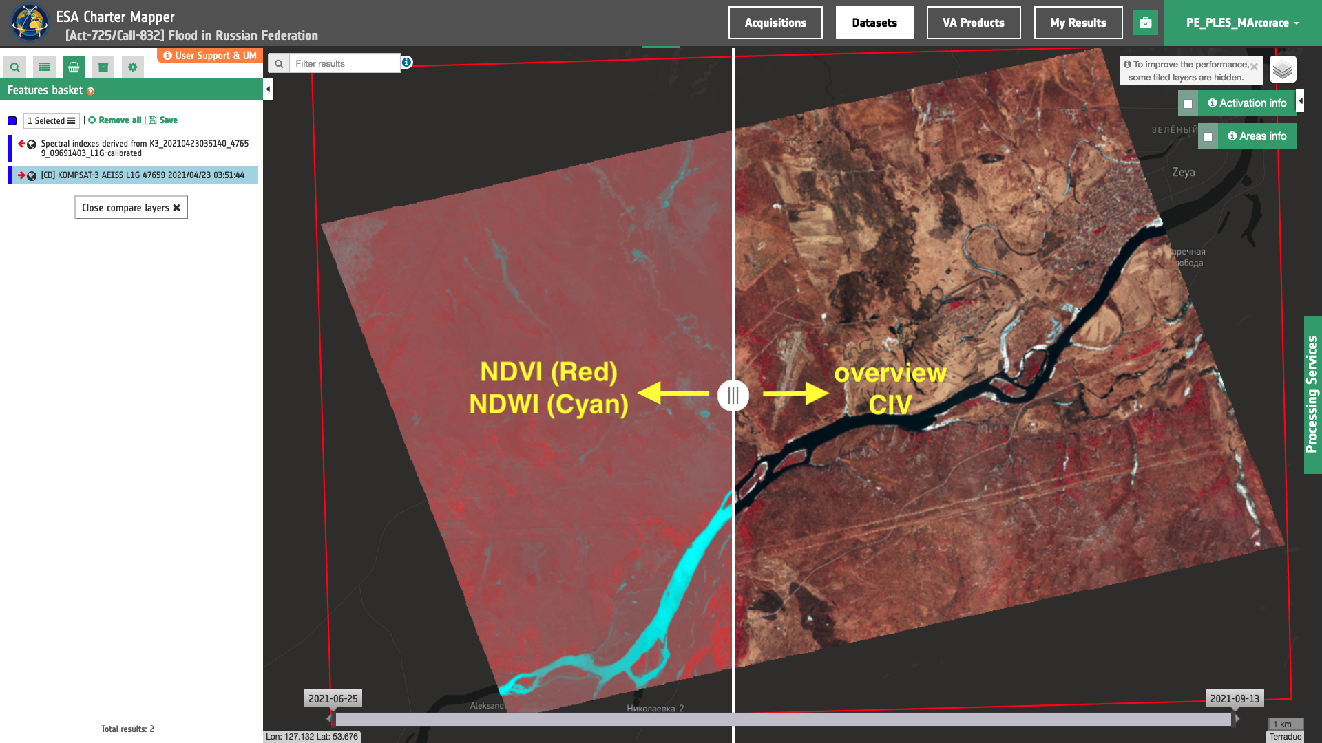
Figure 9 - An example of Spectral Index Product and source Calibrated Dataset stored into the Feature Basket (Image credit: KARI).

Once in the Feature Basket the user can also visually compare NDVI with the TOA reflectance by selecting the two layers and clicking on the Compare Layers function. A vertical slider bar will appear as shown in Figure 10.

Figure 10 - Visual comparison of Red-Cyan composite of NDVI and NDWI with the CIV overview using the slider bar in the ESA Charter Mapper (Image credit: KARI).

The below silent video explains how to compare input and outputs from a processing service by dragging and dropping items in the feature basket and creating a data package.

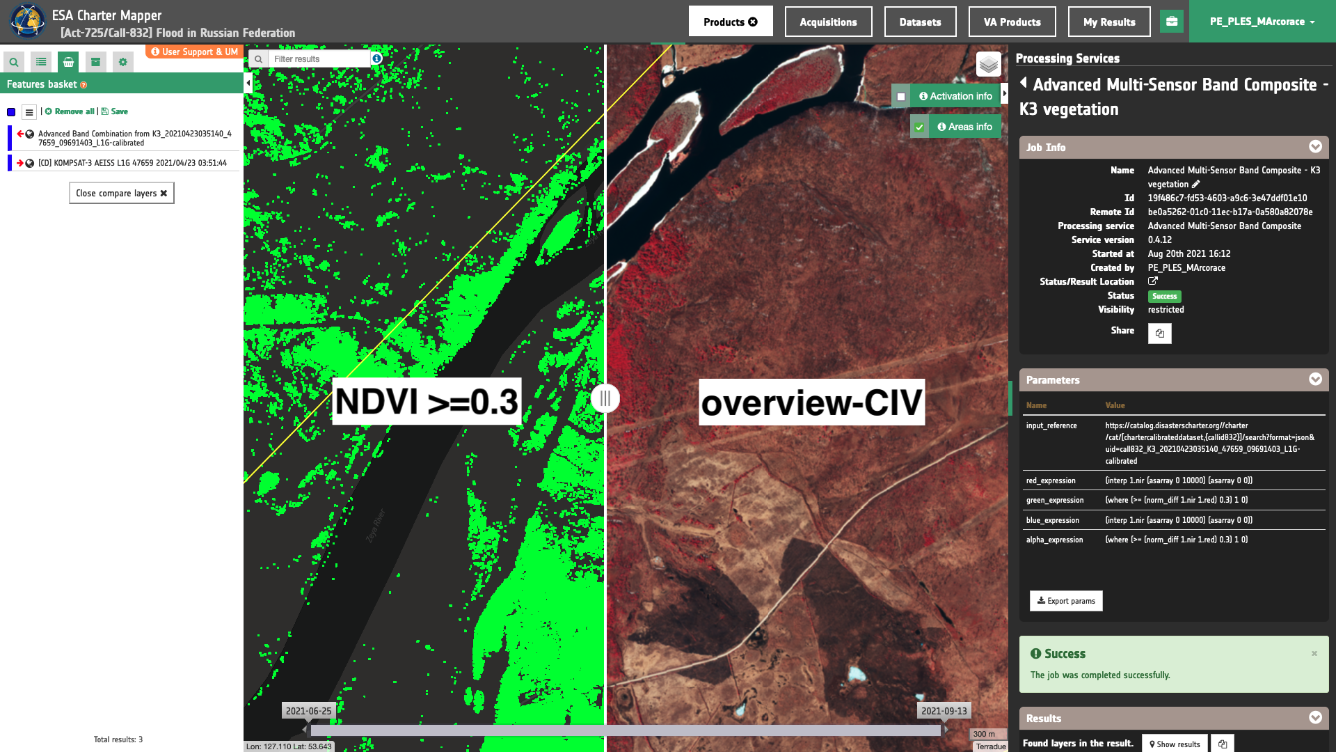
ESA Charter Mapper Features Basket and Data packages panel silent video

In a similar manner to better assess vegetated areas, a binary mask in green obtained from the Advanced Multi Sensor Composite (COMBI-Plus) service can be also visually compared with the Color Infrared Vegetation RGB composite obtained from the same Kompsat-3 data. More information about the Advanced Multi Sensor Composite service function can be found by looking at the COMBI-Plus tutorial as well as the COMBI-Plus service specifications.

figure 10B

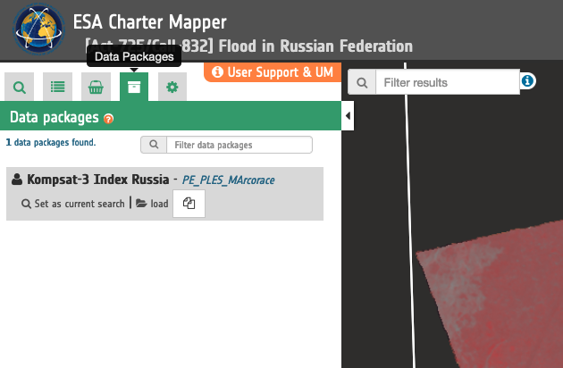
These products can also be saved into a Data Package to be shared among authorized users (e.g. from PM to a VA). The procedure for the creation of a Data Package in the ESA Charter Mapper from the two selected features of the Calibrated Dataset and the Spectral Index product from Kompsat-3 data is shown in the below Figures 11 and 12.

Figure 11 - The procedure for the creation of a Data Package in the ESA Charter Mapper from selected features in the Feature Basket (Image credit: KARI).

Figure 12 - The Data Package tab showing the Data Package just created from Kompsat-3 data in the ESA Charter Mapper (Image credit: KARI).