Auxiliary data
Base layers from auxiliary data
Different auxiliary datasets are offered in the ESA Charter Mapper as static layers to be used only for visualisation purposes as alternative (or complementary) base layers to the default one.
The list of auxiliary data base layers that are available is the following:
-
Copernicus DEM1
-
ESA World Cover2
-
JRC Global Surface Water3,4 (Transitions, Change, Seasonality, Recurrence, Extent, Occurrence),
-
DLR World Settlement Footprint 20195
-
NASA Gridded Population of the World 20206
The below figure shows an example of visualisation of the ESA World Cover Base layer in the map.
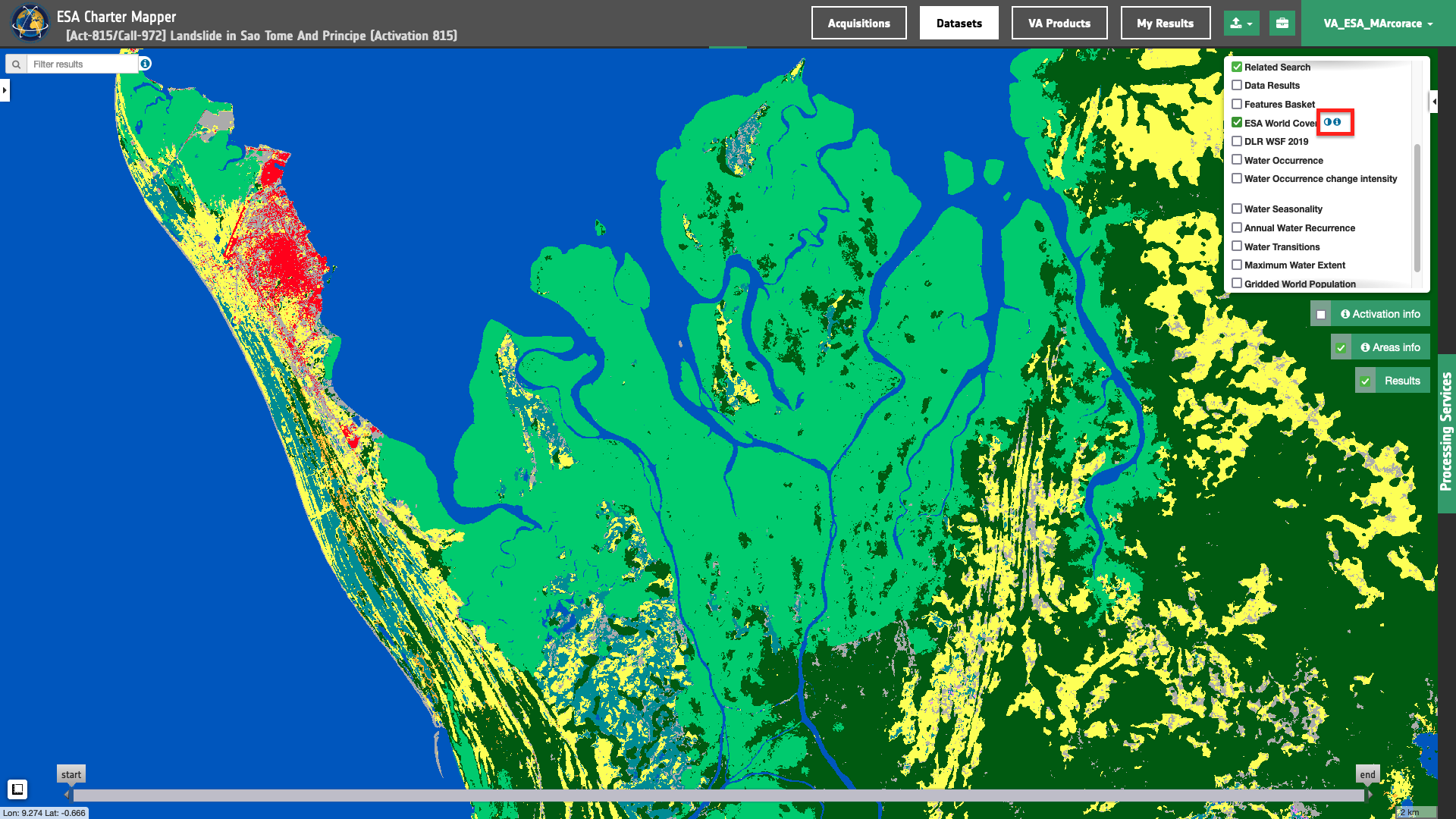
Using the show layer info button next to the title of the layer in the list it is possible to superimpose each auxiliary base layer to the default basemap by setting a desired level of transparency.
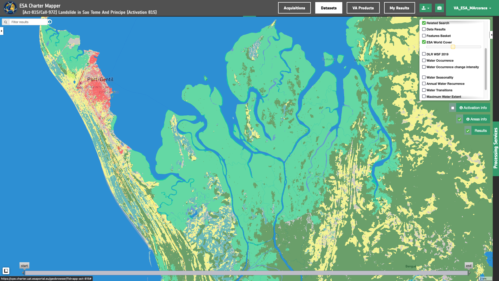
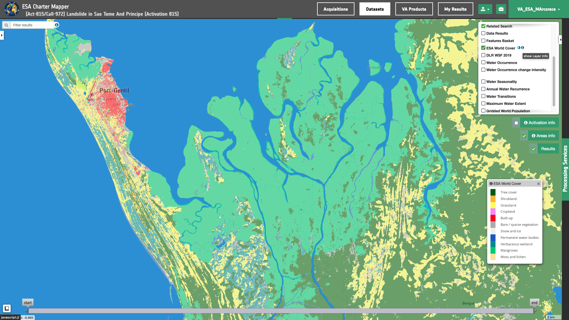
For each base layer it is also possible to display the related legend by clicking on the show layer info button.
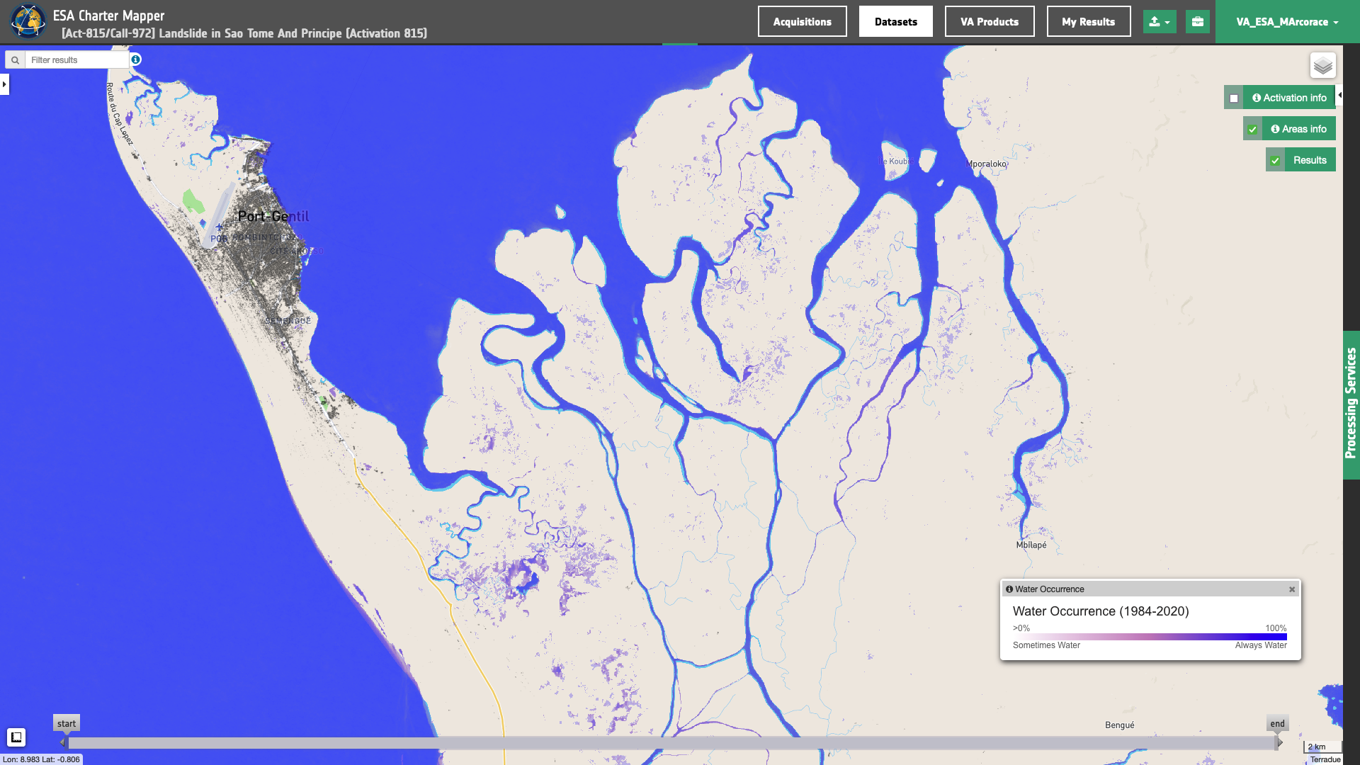
Opacity can be also used to superimpose multiple auxiliary data layers, as shown in the below figure between the GSW Water Occurrence and the WSF 2019 layers near the Gabon coast.
Warning
The ESA Charter Mapper relies on the external map / tile servers provided by the providers of the Auxiliary datasets.
Auxiliary Datasets
The ESA Charter Mapper also offers auxiliary data in the form of Datasets including single or multiple assets to be used for visualization and processing.
List of offered Auxiliary Datasets
Selected Auxiliary Datasets are the following:
-
Copernicus DEM1,
-
ESA Global Land Cover 20202,
-
World Settlement Footprint 20195,
-
WorldPop Population Counts 20207.
Each dataset includes a single band asset and its overview. The overview asset is the one visualized by default in the map. The list of Auxiliary Datasets and their single band assets is given in Table 1.
| Auxiliary Dataset | Description | Single Band Asset | Res (m) |
|---|---|---|---|
| Copernicus DEM | (GLO-30) DSM with global coverage and resolution of 30m. Absolute vertical accuracy < 4m (90% linear error). Absolute horizontal accuracy < 6m (90% circular error) | cop-dem |
30 |
| ESA WorldCover 2020 | Land Cover for 2020 from S1 and S2 data | worldcover |
10 |
| Global Surface Water 1984-2020 - Occurrence | Shows where surface water occurred between 1984 and 2020 and provides information concerning overall water dynamics. This product captures both the intra and inter-annual variability and changes. | gsw-occurrence |
25 |
| Global Surface Water 1984-2020 - Occurrence Change Intensity | Provides information on where surface water occurrence increased, decreased or remained the same between 1984-1999 and 2000-2020. | gsw-change |
25 |
| Global Surface Water 1984-2020 - Seasonality | Provides information concerning the intra-annual behaviour of water surfaces for a single year (2020) and shows permanent and seasonal water and the number of months water was present. | gsw-seasonality |
25 |
| Global Surface Water 1984-2020 - Recurrence | Provides information concerning the inter-annual behaviour of water surfaces and captures the frequency with which water returns from year to year. | gsw-recurrence |
25 |
| Global Surface Water 1984-2020 - Transitions | Provides information on where surface water occurrence increased, decreased or remained the same between 1984-1999 and 2000-2020. | gsw-transitions |
25 |
| Global Surface Water 1984-2020 - Extent | Provides information on where surface water occurrence increased, decreased or remained the same between 1984-1999 and 2000-2020. | gsw-extent |
25 |
| World Settlement Footprint 2019 | Binary mask outlining the extent of human settlements globally (2019) | wsf_2019 |
10 |
| WorldPop 2020 | Population Counts UN Adjusted 2020 | world-pop |
100 |
| HAND | Height Above the Nearest Drainage from the MERIT-Hydro dataset | hand |
90 |
Table 1 - Single band assets included into Auxiliary datasets.
Names of Single Band asset listed in Table 1 refers also to STAC keys. Those keys (e.g. cop-dem for the Copernicus DEM Auxiliary Dataset) are the ones to be used when employing a single band asset from an Auxiliairy Dataset into on-demand processing (e.g. in the STACK service).
Systematic Dataset creation for the activation workspace
For the auxiliary datasets to be made available for processing, the data in its original format is gathered from the source, either external or from a local repository, pre-processed to convert it in the format needed by the processing services (STAC+COG) and stored in the Activation storage space. This ensures its availability and usability for the full duration of the activation. Their reformatting in STAC+COG also enables visualisation via the platform tiler (i.e. the layer styling function).
Once an activation workspace is created, a background processing implements a mosaic over the call areas buffered envelope. As an example in the case of the areas defined in the [Act-756/Call-869] Tropical Storm Megi in the Philippines, the auxiliary datasets offered within the workspace do not have a global extension but cover only the portion of the Philippines surrounding the activation areas.
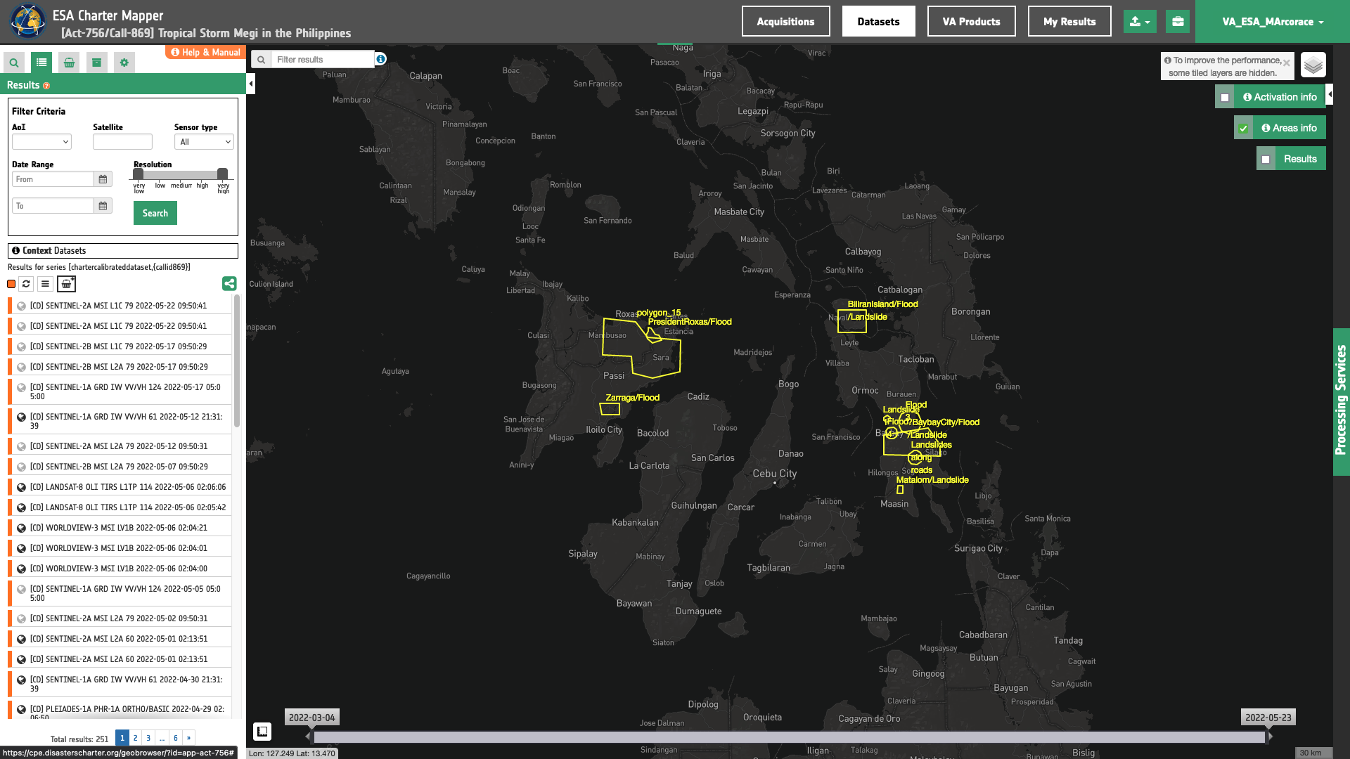
In particular, the creation of a mosaic for each auxiliary dataset is done by using a buffered polygon including all activation areas as shown in the below figure.
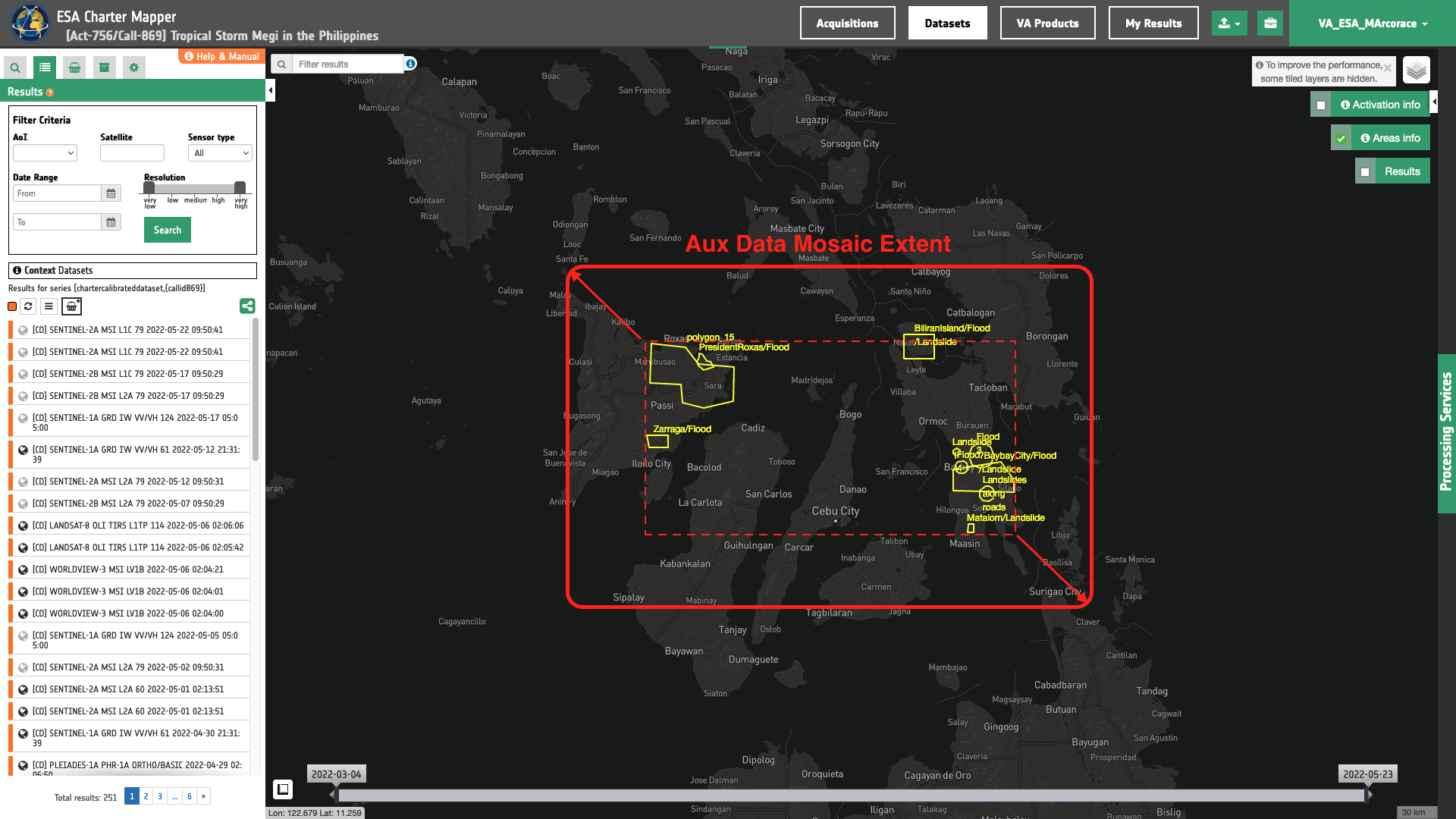
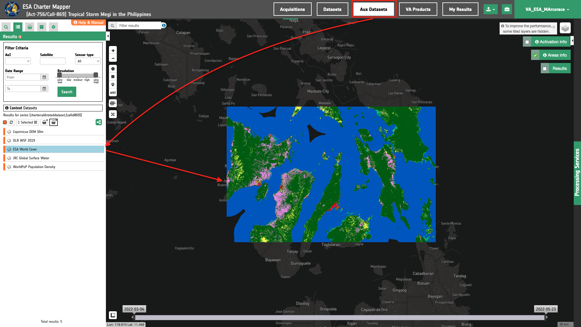
This polygon buffered with a certain distance (e.g. 0.05 degrees) is then used to select all the intersecting tiles. Therefore the resulting mosaic includes a wider area than the one shown in the below image with the rectangle in white. The mosaicking is triggered one by one systematically for all auxiliary datasets. Thus, in the activation workspace the users access a list of Auxiliary Datasets by clicking on the Aux Datasets data context upper menu.
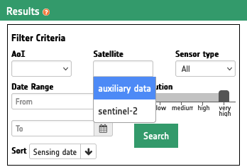
Warning
The Aux Datasets data context button in the upper menu is currently under development. Thus, Auxiliary Datasets can temporarly found under Datasets. In this temporary situation please note that to filter Auxiliary Datasets from Calibrated EO Datasets in the Filter Criteria under the Satellite filter use the class auxiliary data.
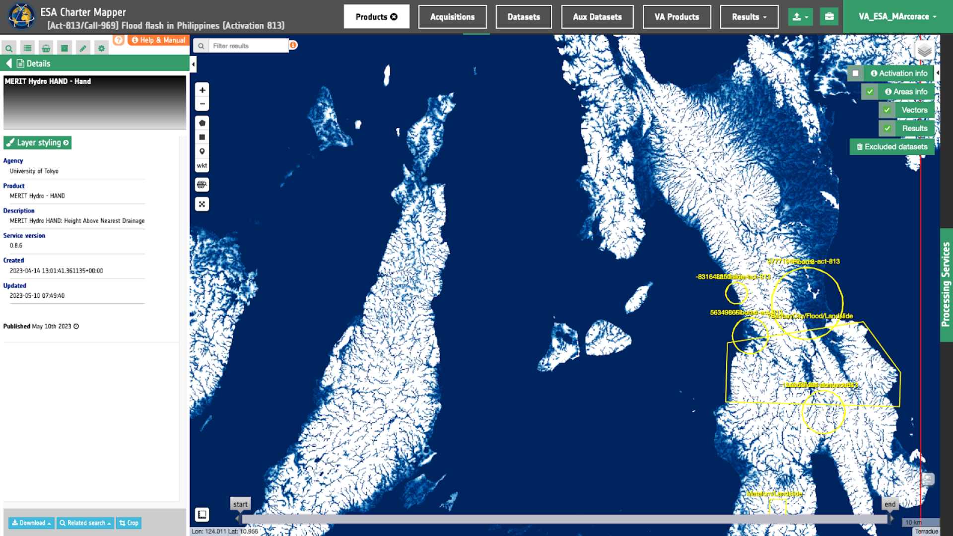
Once the mosaicking is done and all resulting auxiliary datasets are published, PM/VAs can easily visualise the asset in the map at full resolution, change layer styling and consult the values directly in the map as shown in the below figure.
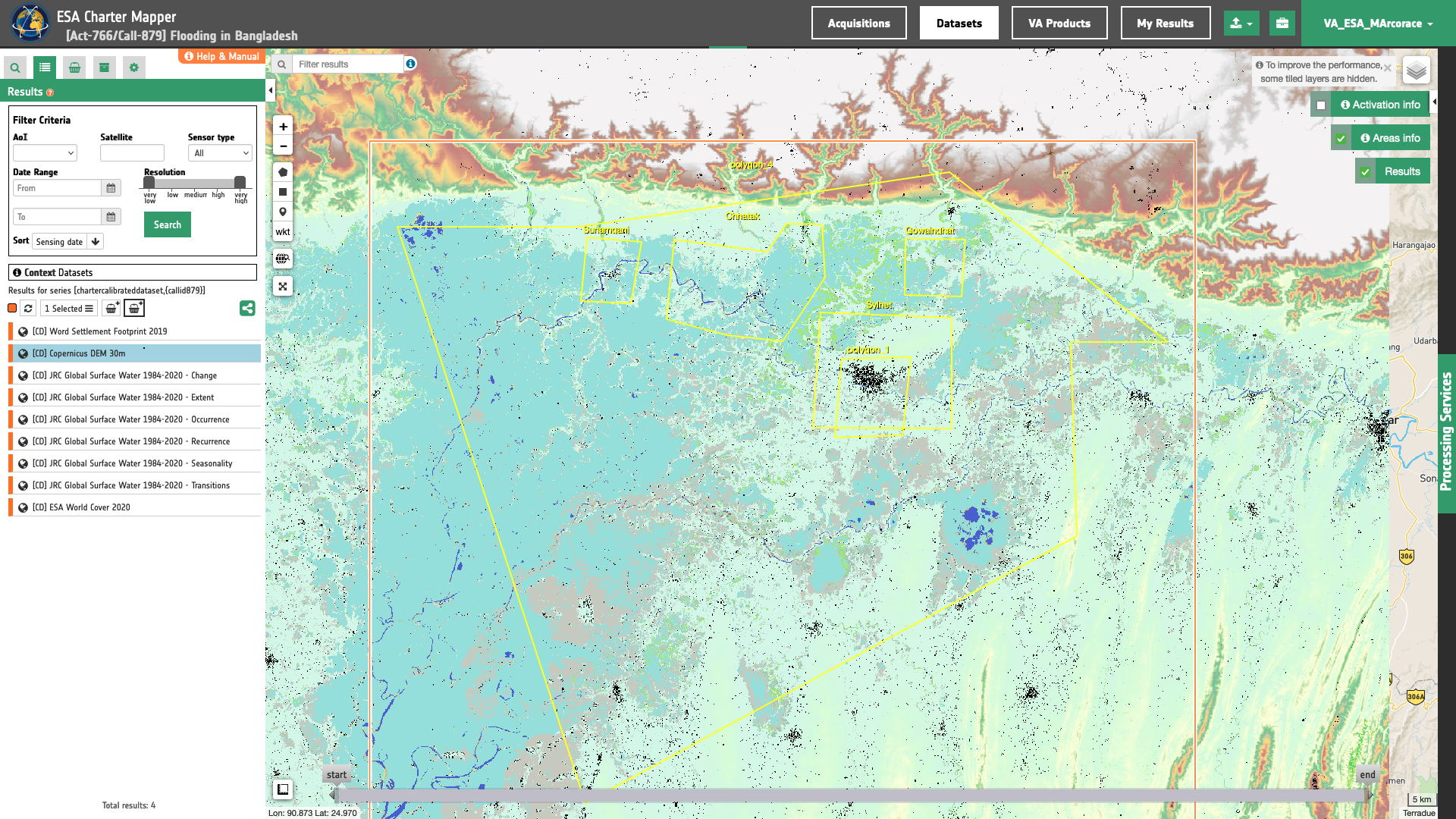
Auxiliary Datasets appear as multiple features under Results in the left panel as shown in the below image.
After selecting one of the features in the result list the user can see in the map each auxiliary dataset one by one. In a similar manner the user can drag and drop the selected Dataset as input to a processing service (when relevant and supported by the processing service).
Specifications for each single band asset included in Auxiliary Datasets can be found in the below sections.
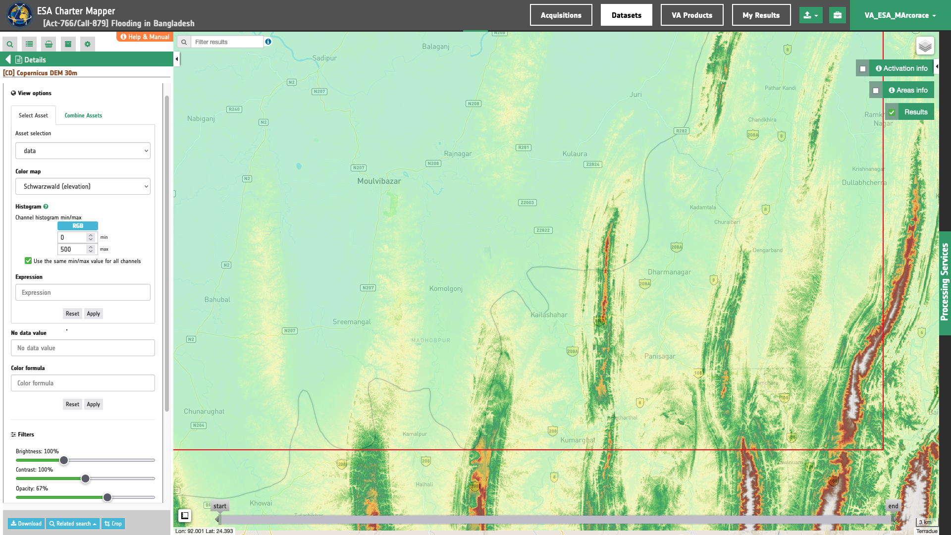
Copernicus DEM single band asset specifications
The cop-dem asset is given as a single band Float32 raster in COG format. Pixel size of 0.0003 deg. Pixel values represent elevation in meters.
Warning
The overview asset is not included in the Copernicus DEM Auxiliary Dataset.
Tip
For a better visualization of the cop-dem single band asset elevation in the map it is possible under Layer Styling to employ a schwarzwald color map and make an image stretching, by changing min/max elevation values from histogram panel.
ESA World Cover single band asset specifications
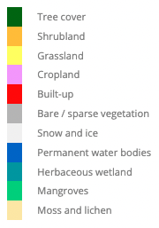
The worldcover asset is given as a single band 8-bit unsigned integer raster in COG format. Pixel size of 0.0001 deg. In Table 2 are given definitions and pixel values for all the 11 LC classes.
| Pixel Value | Land Cover Class | Definition |
|---|---|---|
| 10 | Tree cover | This class includes any geographic area dominated by trees with a cover of 10% or more. Other land cover classes (shrubs and/or herbs in the understorey, built-up, permanent water bodies, ...) can be present below the canopy, even with a density higher than trees. Areas planted with trees for afforestation purposes and plantations (e.g. oil palm, olive trees) are included in this class. This class also includes tree covered areas seasonally or permanently flooded with fresh water except for mangroves. |
| 20 | Shrubland | This class includes any geographic area dominated by natural shrubs having a cover of 10% or more. Shrubs are defined as woody perennial plants with persistent and woody stems and without any defined main stem being less than 5 m tall. Trees can be present in scattered form if their cover is less than 10%. Herbaceous plants can also be present at any density. The shrub foliage can be either evergreen or deciduous |
| 30 | Grassland | This class includes any geographic area dominated by natural herbaceous plants (Plants without persistent stem or shoots above ground and lacking definite firm structure): (grasslands, prairies, steppes, savannahs, pastures) with a cover of 10% or more, irrespective of different human and/or animal activities, such as: grazing, selective fire management etc. Woody plants (trees and/or shrubs) can be present assuming their cover is less than 10%. It may also contain uncultivated cropland areas (without harvest/ bare soil period) in the reference year. |
| 40 | Cropland | Land covered with annual cropland that is sowed/planted and harvestable at least once within the 12 months after the sowing/planting date. The annual cropland produces an herbaceous cover and is sometimes combined with some tree or woody vegetation. Note that perennial woody crops will be classified as the appropriate tree cover or shrub land cover type. Greenhouses are considered as built-up. |
| 50 | Built-up | Land covered by buildings, roads and other man-made structures such as railroads. Buildings include both residential and industrial building. Urban green (parks, sport facilities) is not included in this class. Waste dump deposits and extraction sites are considered as bare. |
| 60 | Bare / sparse vegetation | Lands with exposed soil, sand, or rocks and never has more than 10 % vegetated cover during any time of the year. |
| 70 | Snow and ice | This class includes any geographic area covered by snow or glaciers persistently. |
| 80 | Permanent water bodies | This class includes any geographic area covered for most of the year (more than 9 months) by water bodies: lakes, reservoirs, and rivers. Can be either fresh or salt-water bodies. In some cases the water can be frozen for part of the year (less than 9 months). |
| 90 | Herbaceous wetland | Land dominated by natural herbaceous vegetation (cover of 10% or more) that is permanently or regularly flooded by fresh, brackish or salt water. It excludes unvegetated sediment (see 60), swamp forests (classified as tree cover) and mangroves see 95). |
| 95 | Mangroves | Taxonomically diverse, salt-tolerant tree and other plant species which thrive in intertidal zones of sheltered tropical shores, "overwash" islands, and estuaries. |
| 100 | Moss and lichen | Land covered with lichens and/or mosses. Lichens are composite organisms formed from the symbiotic association of fungi and algae. Mosses contain photo-autotrophic land plants without true leaves, stems, roots but with leaf-and stemlike organs. |
Table 2 - Definition of classes for the single band asset of the ESA World Cover auxiliary dataset.
Pixel value of 0 represents No Data.
In the worldcover_overview asset LC classes are visualized in the map using the color schema shown in the below legend.
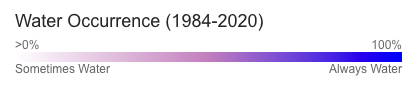
GSW Water Occurrence single band asset specifications
The gsw-occurrence asset is given as a single band 8-bit unsigned integer raster in COG format. Pixel size of 0.00025 deg. Table 3 describes pixel values for this asset which represents occurrence value expressed as a percentage.
| Pixel Value | Label |
|---|---|
| 0 | Not water |
| 1 | 1% Occurrence |
| 100 | 100% Occurrence |
| 255 | No data |
Table 3 - Values for the single band asset of the GSW 1984-2020 Water Occurrence auxiliary dataset.
In the gsw-occurrence_overview asset, water occurrence is visualized in the map using the color schema shown in the below legend.
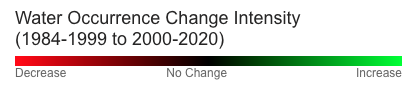
GSW Water Occurrence Change Intensity single band asset specifications
The gsw-change asset is given as a single band 8-bit unsigned integer raster in COG format. Pixel size of 0.00025 deg. Table 4 describes pixel values for this asset which represents the normalised difference in the mean occurrence value between the two epochs for homologous months epoch1-epoch2 /epoch1+epoch2.
| Pixel Value | Label |
|---|---|
| 0 | -100% loss of occurrence |
| 100 | No change |
| 200 | 100% increase in occurrence |
| 253 | Not water |
| 254 | Unable to calculate a value due to no homologous months |
| 255 | No data |
Table 4 - Values for the single band asset of the GSW 1984-2020 Water Occurrence Change Intensity auxiliary dataset.
In the gsw-change_overview asset, water occurrence change intensity is shown in the map using the color schema shown in the below legend.
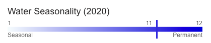
GSW Seasonality single band asset specifications
The gsw-change asset is given as a single band 8-bit unsigned integer raster in COG format. Pixel size of 0.00025 deg. Table 5 describes pixel values for this asset which represents the number of months that water was present from January 2020 to December 2020.
| Pixel Value | Label |
|---|---|
| 0 | Not water |
| 1 | 1 month of water |
| 12 | 12 months of water (permanent water) |
| 255 | No data |
Table 5 - Values for the single band asset of the GSW 1984-2020 Seasonality auxiliary dataset.
In the gsw-seasonality_overview asset, occurrence change intensity is shown in the map using the color schema shown in the below legend.
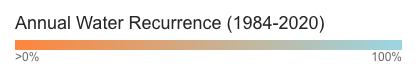
GSW Recurrence single band asset specifications
The gsw-recurrence asset is given as a single band 8-bit unsigned integer raster in COG format. Pixel size of 0.00025 deg. Table 6 describes pixel values for this asset which represents the frequency with which water returns from years to year expressed as a percentage.
| Pixel Value | Label |
|---|---|
| 0 | Not water |
| 1 | 1% recurrence |
| 100 | 100% recurrence |
| 255 | No data |
Table 6 - Values for the single band asset of the GSW 1984-2020 Recurrence auxiliary dataset.
In the gsw-recurrence_overview asset, annual water recurrence is shown in the map using the color schema shown in the below legend.
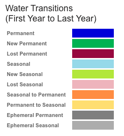
GSW Transitions single band asset specifications
The gsw-transitions asset is given as a single band 8-bit unsigned integer raster in COG format. Pixel size of 0.00025 deg. Table 7 describes pixel values for this asset which represents the type of transition between the first and last year.
| Pixel Value | Label |
|---|---|
| 0 | Not water |
| 1 | Permanent |
| 2 | New permanent |
| 3 | Lost permanent |
| 4 | Seasonal |
| 5 | New seasonal |
| 6 | Lost seasonal |
| 7 | Seasonal to permanent |
| 8 | Permanent to seasonal |
| 9 | Ephemeral permanent |
| 10 | Ephemeral seasonal |
| 255 | No data |
Table 7 - Values for the single band asset of the GSW 1984-2020 Transitions auxiliary dataset.
In the gsw-transitions_overview asset, water transitions is shown in the map using the color schema shown in the below legend.
GSW Water Extent single band asset specifications
The gsw-extent asset is given as a single band 8-bit unsigned integer raster in COG format. Pixel size of 0.00025 deg. Table 2 describes pixel values for this asset which represents a simple flag indicating if water was detected or not.
| Pixel Value | Label |
|---|---|
| 0 | Not water |
| 1 | Water detected |
| 255 | No data |
Table 8 - Values for the single band asset of the GSW 1984-2020 Water Extent auxiliary dataset.
In the gsw-extent_overview asset, water extent is visualized in the map in blue (using colour #6666FF).
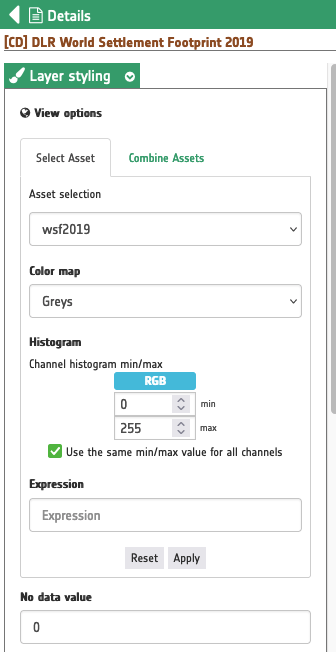
World Settlement Footprint single band asset specifications
The wsf2019 asset is given as a single band 8-bit unsigned integer raster in COG format. Pixel size of 0.0001 deg. Pixel value of 0 represents No Data. Pixel value of 255 represent the true value.
Warning
The overview asset is not included in the World Settlement Footprint 2019 Auxiliary Dataset.
Tip
For a better visualization of the wsf2019 single band asset in the map it is possible under Layer Styling to change default View options and apply the following:
-
Asset selection:
wsf2019 -
Color map:
Greys -
Histogram: Channel histogram min =
0, max =255 -
No data value:
0
WorldPop Population Counts single band asset specifications
The world-pop asset is given as single band Float32 raster in COG format. Pixel size of 0.0008 deg. Pixel values represent population counts over a 100x100m square pixel area. Value of -99999 represents No Data.
Warning
The overview asset is not included in the WorldPop Population Counts 2020 Auxiliary Dataset.
Tip
For a better visualization of the world-pop single band asset in the map it is possible under Layer Styling to change default View options and apply the following:
-
Asset selection:
world-pop -
Color map:
Viridis -
Histogram: Channel histogram min =
0, max =1000
HAND single band asset specifications
The hand single band asset is given as a single band Float32 raster in COG format. It is taken from the MERIT-Hydro Aux Dataset developed by the University of Tokyo. Pixel size of 0.00008333 deg. The undefined pixels (oceans) are represented by the value -9999. Pixel values represent Height Above the Nearest Drainage in meters derived from the hydrologically conditioned MERIT DEM.
Tip
For the visualization of the hand single band asset in the map it is possible under Layer Styling to change default View options and apply the following:
-
Asset selection:
hand -
Color map:
Blues -
Histogram: Channel histogram min =
0, max =15
The hand-overview overview asset shows heights above the nearest drainage in blue (0m) to white shades (10m) derived from the MERIT-Hydro Aux Dataset. This visual asset is given as a multi-band 8bit raster in COG format
-
Copernicus DEM global 30m (GLO-30) DSM at 30m resolution. More info at: spacedata.copernicus.eu. ↩↩
-
ESA World Cover, global land cover product at 10 m resolution for 2020 based on Sentinel-1 and 2 data with 11 LC classes. More info at: esa-worldcover.org. ↩↩
-
Pekel, JF., Cottam, A., Gorelick, N. et al. High-resolution mapping of global surface water and its long-term changes. Nature 540, 418–422 (2016). DOI: 10.1038/nature20584. ↩↩
-
Global Surface Water 1984-2020, Occurrence, Occurrence change intensity, Seasonality, Recurrence, Transitions, and Maximum water extent. More info at: global-surface-water.appspot.com. ↩↩
-
DLR World Settlement Footprint 2019. More info at: www.dlr.de. ↩↩
-
Gridded Population of the World 2020, distribution of human population (counts and densities) on a continuous global raster surface. More info at: sedac.ciesin.columbia.edu. ↩
-
Population density 2020 UN adjusted GeoTIFF at 100m resolution. More info at: www.worldpop.org. ↩
-
Nobre, Antonio & Cuartas, Luz & Hodnett, M & Rennó, Camilo & Medeiros, Grasiela & Silveira, Andre & Waterloo, M.J. & Saleska, Scott. (2011). Height Above the Nearest Drainage - a hydrologically relevant new terrain model. Journal of Hydrology. 404. 13-29. DOI:[10.1016/j.jhydrol.2011.03.051] https://doi.org/10.1016/j.jhydrol.2011.03.051{:target="_blank"}. ↩
-
Yamazaki, D., Ikeshima, D., Sosa, J., Bates, P. D., Allen, G. H., & Pavelsky, T. M. (2019). MERIT Hydro: a high-resolution global hydrography map based on latest topography dataset. Water Resources Research, 55, 5053– 5073. DOI:10.1029/2019WR024873. ↩