NDVI Change Detection service specifications

The service first performs a co-registration of a pair optical calibrated datasets acquired before and after an event. Then, it derives a binary change mask from the NDVI difference by using a threshold and a spatial filter. The output is a binary map representing the NDVI loss, given in raster and vector formats. The input datasets may come from different optical sensors.

The tutorial of the NDVI-CD service is available in this section.

Service Description

The NDVI Change Detection (NDVI-CD) processing service takes a pair of multi-mission optical calibrated datasets acquired before and after an event (e.g. wildfire, landslide), makes a co-registration of nir and red assets, estimates the loss of NDVI¹ by doing first a binarization of the difference in NDVI between post- and pre-event datasets. NDVI loss products in raster and vector format are then obtained after a spatial filtering of the binary raster and a conversion to polygon vector.

cover

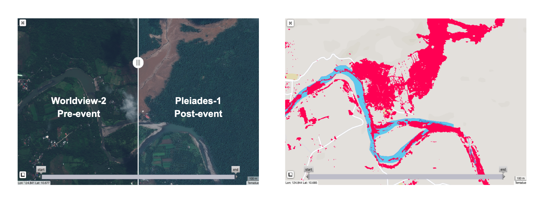
Figure 1 - NDVI loss due to a large landslide in Baybay, Philippines, Apr 2022

Tip

With NDVI loss we refer to a drop of greenness in the post-event images with respect to the reference (pre-event).

Note

In image processing, binarization thresholding is a simple image segmentation method in which all images are assigned to a value of 0 (false) or 1 (true).

Workflow

The NDVI-CD service implements the workflow depicted below.

graph TB b[(Calibrated Datasets)] style b fill:#ffde86,stroke:#333,color:#282828,stroke-width:2px b --> a1[input 1] b --> a2[input 2] subgraph Input style Input fill:#e8e8e8,stroke:#818181,color:#282828 a1[/Dataset Pre/] style a1 fill:#acc8ff,stroke:#333,color:#282828,stroke-width:2px a2[/Dataset Post/] style a2 fill:#acc8ff,stroke:#333,color:#282828,stroke-width:2px a3[/AOI as WKT/] style a3 fill:#acc8ff,stroke:#333,color:#282828,stroke-width:2px a4[/Reference asset/] style a4 fill:#acc8ff,stroke:#333,color:#282828,stroke-width:2px a5[/Filter threshold/] style a5 fill:#acc8ff,stroke:#333,color:#282828,stroke-width:2px a6[/NDVI threshold/] style a6 fill:#acc8ff,stroke:#333,color:#282828,stroke-width:2px end subgraph NDVI Change Detection a1 --> stack[Co-location] a2 --> stack[Co-location] a3 --> stack[Co-location] stack --> cs1(Co-located red_pre) style cs1 fill:#cfdfff,stroke:#333,color:#282828 stack --> cs2(Co-located red_post) style cs2 fill:#cfdfff,stroke:#333,color:#282828 stack --> cs3(Co-located nir_pre) style cs3 fill:#cfdfff,stroke:#333,color:#282828 stack --> cs4(Co-located nir_post) style cs4 fill:#cfdfff,stroke:#333,color:#282828 cs1 --> cloudmask[Cloud Masking] cs2 --> cloudmask[Cloud Masking] cs3 --> cloudmask[Cloud Masking] cs4 --> cloudmask[Cloud Masking] cloudmask --> coreg[Co-registration] a4 --> coreg[Co-registration] coreg --> ds1(Reference red and nir assets) style ds1 fill:#cfdfff,stroke:#333,color:#282828 coreg --> ds2(Co-registered red and nir assets) style ds2 fill:#cfdfff,stroke:#333,color:#282828 ds1 --> arithm[NDVI loss calculation] ds2 --> arithm[NDVI loss calculation] a6 --> arithm[NDVI loss calculation] arithm --> fil[Filter] a5 --> fil[Filter] fil --> overview[Overview creation] fil --> vec[Vectorize] end subgraph Output style Output fill:#e8e8e8,stroke:#818181,color:#282828 ds1 --> o1[/Reference red and nir assets/] style o1 fill:#acc8ff,stroke:#87afff,color:#282828,stroke-width:2px ds2 --> o2[/Co-registered red and nir assets/] style o2 fill:#acc8ff,stroke:#87afff,color:#282828,stroke-width:2px arithm[NDVI loss calculation] --> o3[/NDVI loss single band/] style o3 fill:#acc8ff,stroke:#87afff,color:#282828,stroke-width:2px fil[Filter] --> o4[/NDVI loss filtered single band/] style o4 fill:#acc8ff,stroke:#87afff,color:#282828,stroke-width:2px overview[Overview creation] --> o5[/NDVI loss overview/] style o5 fill:#acc8ff,stroke:#87afff,color:#282828,stroke-width:2px vec[Vectorize] --> o6[/NDVI loss vector/] style o6 fill:#acc8ff,stroke:#87afff,color:#282828,stroke-width:2px end

Pre processing

From the input pre- and post-event optical calibrated dataset defined by the user, the service first automatically extract red and nir single band assets:

red_pre which stands for the single band reflectance asset having CBN equal to red extracted from the pre-event calibrated dataset,
nir_pre which stands for the single band reflectance asset having CBN equal to nir, or nir08 extracted from the pre-event calibrated dataset,
red_post which stands for the single band reflectance asset having CBN equal to red extracted from the post-event calibrated dataset,
nir_post which stands for the single band reflectance asset having CBN equal to nir, or nir08 extracted from the post-event calibrated dataset.

If input calibrated datasets are from Sentinel-2 L1C or L2A data, the processor masks reflectance with a cloud mask (single band asset CLM) derived from the S2-Cloudless processor within the systematic Optical Image Calibration). The CLM single band asset is derived from a Sentinel-2 calibrated dataset using the S2-Cloudless processor with default parameters as described in here.

Note

Default parameters for S2-Cloudless processor are: Cloud probability threshold to mask cloudy pixels equal to 0.4 for L1C and 0.5 for L2A, Size of the disk in pixels to perform convolution equal to 4, Size of the disk in pixels to perform dilation equal to 2.

Warning

Cloud masking in NDVI-CD is currently available ONLY for Sentinel-2 datasets. No cloud masking is applied to other optical sensors supported by the ESA Charter Mapper. When cloud masking is not applied, the NDVI loss estimation over cloudy areas is biased by low values of the index.

Image stacking and co-registration

Later, it creates a co-located stack of these four single band assets. This co-located stack is then passed to the co-registration software.

The NDVI-CD service employs the GeFolki²,³ coregistration software⁴,⁵ developed at ONERA in the Multidate Earth observation Datamass for Urban Sprawl Aftercase (MEDUSA) project. In NDVI-CD GeFolki is employed with typical parameters for optical flow computation with homogenous data:

\[ u, v = GeFolki ( master, slave, K, r, R, L ) \]

where:

master is the single band asset defined by the user which is assigned in GeFolki as a reference image (e.g. red-post).
slave is the single band asset having the same CBN from the other calibrated dataset which is assigned in GeFolki as a secondary image (e.g. red-pre).
R is the radius, describes the size of the local window on which the correlation between the two images is maximized, which is set equal to [16,8],
L is the number of levels in the scale pyramids. In NDVI-CD this parameter and is set equal to 5,
K is the number of iterations used in the gradient method dedicated to the minimum search, which is set equal to 4,
R is the parameter for the rank filter, which is set equal to 4 (9x9 window).

The optical flow computation with GeFolki is applied once in NDVI-CD and the u,v displacement obtained is then applied to transform both nir and red secondary assets (e.g. red-pre and nir-pre).

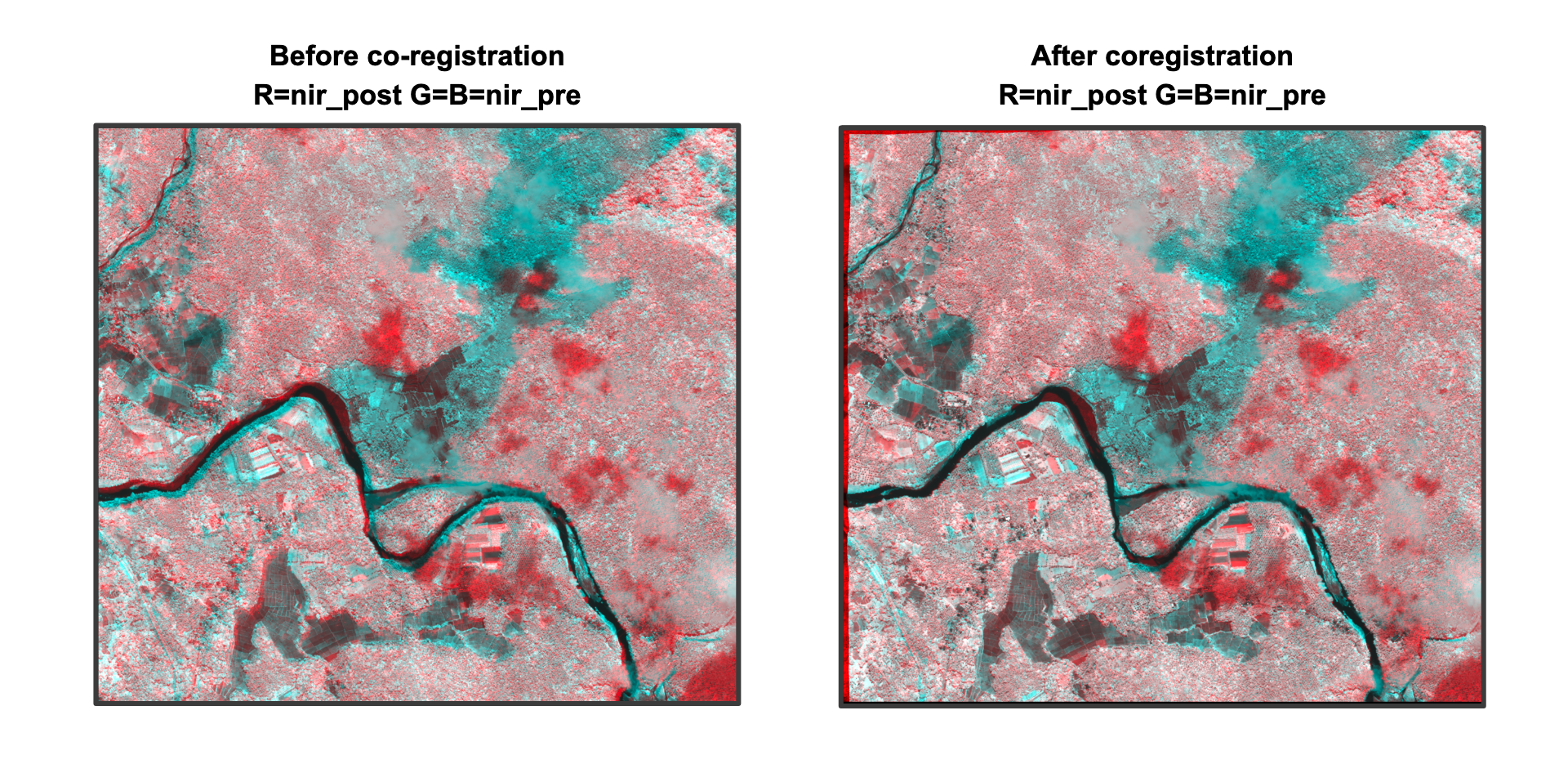
Figure 2 - Example of co-registration of NIR pre- and post-event single band assets using u,v displacement derived from the red ones. Pre-event calibrated data acquired from WorldView-2 and Post-event data acquired from Pleiades over Baybay, Philippines. Image credits: USGS, DigitalGlobe, CNES, Airbus DS

Note

The choice of a red or a nir reference single band asset, defines the flow computation in GeFolki. As an example if a red single band is chosen as reference the u,v displacement to warp secondary red asset is also applied to warp the nir one.

Note

When the co-location and co-registration is made using multi-mission calibrated datasets (e.g. Pleiades VS Sentinel-2), all RED and NIR have the finest resolution.

Binarization of the difference of NDVI before and after the event

After the co-registration, the service computes the difference of NDVI before and after the event from the pairs of nir and red co-registered assets. The difference of NDVI is derived with:

\[ NDVI_{difference} = ( NDVI_{post} - NDVI_{pre} ) \]

where:

\[ NDVI_{post} = ( nir_{post} - red_{post} ) / ( nir_{post} + red_{post} ) \]

\[ NDVI_{pre} = ( nir_{pre} - red_{pre} ) / ( nir_{pre} + red_{pre} ) \]

Later the service makes a binarization of negative NDVI difference values to estimate NDVI loss using a negative threshold defined by the user

\[ NDVI_{loss} = where ( ( NDVI_{difference} <= threshold ) , 1 , 0 ) \]

where threshold is a negative decimal value defined by the user (e.g. -0.5).

Tip

In general, rocks and bare soil have an NDVI equal or lower than 0.1 while dense vegetation (e.g. temperate forest) has NDVI of about 0.6. Thus, a loss of vegetation after a landslide (e.g. debris flow) could be roughly estimated by looking at areas showing a medium-high decrease in NDVI of about NDVI_diff = 0.1 - 0.6 = -0.5.

Note

The NDVI difference is assumed by convention as (NDVI_post - NDVI-pre).

Note

Being the service tailored to map NDVI loss, and thus to make a binarization of negative values in (NDVI_post - NDVI-pre) the logical operator is then fixed as <=.

Post processing

The last step of the NDVI-CD workflow employs a spatial filtering of the NDVI loss binary mask. The spatial filtering is made using the Sieve filter with a threshold size equal to the number of pixels defined by the user. The Sieve spatial filter is often used to simplify a classified image having a large amount of small areas. In NDVI-CD service the Sieve filter removes isolated classified pixels using blob grouping and keeps only clusters of contiguous pixels above the minimal area unit. The spatial filtering of input raster is built with the GDAL Sieve utility⁶.

Finally, the portion of the filtered binary mask with pixels having DN equal to 1 (NDVI loss) is then converted to a polygon vector. The vectorization creates vector polygons for all connected regions of pixels in the raster sharing a common pixel value. This step is based on the GDAL Polygonize utility⁷.

Warning

Avoid converting to polygon a noisy or large raster. When possible, define a smaller AOI or employ sufficient spatial filtering on it (above 30 pixels). A conversion of a large or noisy raster may result in a very large vector file (tens or hundreds of Mb) which is difficult to be handled inside or outside the platform (e.g. in a GIS software).

Input

Input of the NDVI-CD is a pair of optical calibrated dataset acquired before and after the event.

Parameters

The NDVI-CD service requires a specified number of mandatory and optional parameters. The list of service parameters are listed in the table below.

Parameter	Description	Required	Default value
Optical pre-event calibrated dataset	Product reference to input pre-event optical calibrated dataset	YES
Optical post-event calibrated dataset	Product reference to input post-event optical calibrated dataset	YES
Area of interest expressed as WKT	Area of interest expressed in Well-known text	YES
Reference asset	Reference single band asset to be used in the u,v displacement computation	YES
NDVI loss threshold	Threshold value as negative decimal number to be used for the binarization of NDVI-post - NDVI-pre	YES
Minimum Connected Pixels	Filter threshold size in number of pixels required to filter out from the NDVI loss binary mask clusters of pixels smaller than this size	YES	`30`

Table 1 - Service parameters for the NDVI-CD processor.

Pre and Post event optical calibrated datasets

The first two mandatory parameters are dedicated to define the input "Pre-event" and "Post-event" Optical Calibrated Datasets. This pair can come from different optical sensors. Input for Optical pre-event calibrated dataset and Optical post-event calibrated dataset parameters are the references to the Calibrated Datasets. The user can fill each parameter via a drag and drop of the calibrated dataset. The system will automatically select the red and nir (or nir08) assets from the given Calibrated Dataset to be used in the computation.

Warning

Pay attention when defining input datasets via the drag and drop. Do not invert post-event with pre-event calibrated datasets.

Warning

The drag and drop of a single-band asset (e.g. red, and nir) is not possible. Users must drag and drop only an Optical Calibrated Dataset (e.g. "[CD] WORLDVIEW-3 MSI L1B 2023-02-07 08:27:05") in the Optical pre-event calibrated dataset and Optical post-event calibrated dataset fields.

Note

When pre- and post-event datasets are acquired from different sensors (e.g. Pleiades for post-event and Sentinel-2 for pre-event) the detection of NDVI loss is affected by different processing levels, geometric corrections (e.g. orthorectified or not) and view angles. Concerning the spatial resolution of the grid used in the detection of changes, the pair of red and nir assets are sampled at the finest resolution.

Area of interest

In this third mandatory parameter the user must define an area of interest within the intersecting area of the two datasets.

Tip

In the definition of “Area of interest as Well Known Text” it is possible to apply as AOI the drawn polygon defined with the area filter. To do so, click on the Magic tool wizard button in the left side of the "Area of interest expressed as Well-known text" box and select the option AOI from the list. The platform will automatically fill the parameter value with the rectangular bounding box taken from the current search area in WKT format.

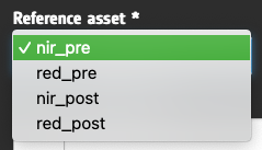
Reference asset

In the fourth parameter the user must define which asset shall be considered as reference in the co-registration. Options are: red_pre, red_post, nir_pre and nir_post.

Being the post-event dataset orthorectified and vegetation changes more sensitive to changes in the NIR, select red_post as reference single band asset.

When choosing a reference asset for the co-registration, the user shall consider:

if the reference need to be taken from the pre- or the post-event dataset (e.g. if one is orthorectified and the other one is not),
in which spectral band (red or nir) the u,v displacement shall be computed (e.g. in the RED channel being vegetation changes more sensitive to variations in the NIR).

NDVI loss threshold

This parameter defines the threshold as a negative decimal value (e.g. -0.5) to be used in the binarization of NDVI difference.

Note

The NDVI difference is assumed by convention as (NDVI_post - NDVI-pre).

Minimum connected pixels

In this parameter the user shall specify a threshold size in pixels to be used in the Sieve Spatial Filtering. As an example 50 means filtering clusters of pixels having size up to 50 pixels.

Minimum and default value: 30
Maximum: N -> there is not a maximum. The higher the number is the bigger is the aggregated number of class clusters

Warning

Threshold value shall be a positive integer number equal or higher than 30.

Tip

To estimate major changes and/or for a quick estimation of NDVI loss employ a medium 50 or high 100 filtering threshold. The vectorization of a medium-high filtered binary raster will be much faster.

Output

The NDVI-CD processor provides in output the following products:

NDVI-CD overview asset (overview-ndvi-change-filtered) showing the NDVI loss in red with transparency, given as multi-band raster in COG format,
NDVI-loss polygon vector in GeoJSON (.json)⁷ and FlatGeoBuf (.fgb)⁸ formats.
NDVI-CD filtered and not filtered single band assets (ndvi-change-filtered, and ndvi-change), given as single-band binary raster in COG format,
Co-registered single band assets pre_red, post_red, pre_nir (or pre_nir08), and post_nir (or post_nir08) derived from pre- and post-event datasets, given as single-band binary raster in COG format,

NDVI-CD Product Specifications can be found in the below tables.

NDVI loss overview

Attribute	Value / description
Description	NDVI change detection map
Short Name	`overview-ndvi-change-filtered`
Description	NDVI loss bitmask in the red channel with transparency
Geospatial Data Type	Raster
Data Type	UnSigned 8-bit Integer
Band	4
Format	COG
Projection	Native or EPSG:4326 - WGS84
Valid Range	[1 - 255]
Fill Value	0

NDVI loss filtered single band

Attribute	Value / description
Description	Spatially filtered NDVI loss as binary single band raster
File Name	`ndvi-change-filtered`
Geospatial Data Type	Raster
Data Type	Float32
Band	1
Format	COG
Projection	Native
Fill Value	Native (e.g. 0 for binary mask)

NDVI loss polygon vector

Attribute	Value / description
Description	Polygon vector resulting from the vectorization of NDVI loss single band for pixels having DN=1
Short Name	`result`
Geospatial Data Type	Vector
Vector Data Type	Polygon
Attributes	ID, DN
Format	GeoJson, FlatGeoBuf
Projection	EPSG:3857 - WGS 84 / Pseudo-Mercator

NDVI loss single band

Attribute	Value / description
Description	Not filtered NDVI loss as binary single band raster
File Name	`ndvi-change`
Geospatial Data Type	Raster
Data Type	Float32
Band	1
Format	COG
Projection	Native
Fill Value	Native (e.g. 0 for binary mask)

Input co-registered single band assets

Attribute	Value / description
Description	Co-registered single band assets derived from pre- and post-event datasets
File Name	`pre_red`, `post_red`, `pre_nir` (or `pre_nir08`), and `post_nir` (or `post_nir08`)
Geospatial Data Type	Raster
Data Type	Float32
Band	1
Format	COG
Projection	Native

Rouse J., Haas R. H., Schell J. A., Deering D. (1973), “Monitoring vegetation systems in the great plains with ERTS”, NASA. Goddard Space Flight Center 3d ERTS-1 Symp., Vol. 1, Sect. A. Available at: ntrs.nasa.gov ↩
Plyer, A., et al. (2015), "A New Coregistration Algorithm for Recent Applications on Urban SAR Images", Geoscience and Remote Sensing Letters, IEEE, 12(11), 2198-2202. DOI: 10.1109/LGRS.2015.2455071. ↩
Brigot, G., et al. (2016), "Adaptation and Evaluation of an optical flow method applied to co-registration of forest remote sensing images", accepted with modifications in IEEE Journal of Selected Topics in Applied Earth Observations and Remote Sensing, Volume: 9, Issue7, July 2016. DOI: 10.1109/JSTARS.2016.2578362. ↩
GeFolki GitHub page, available at: https://github.com/. ↩
GeFolki User manual, available at: https://github.com/. ↩
GDAL Sieve Filter and its implementation in QGIS software, GDAL documentation, available at https://gdal.org and at https://docs.qgis.org. ↩
GDAL Polygonize and its implementation in QGIS software, GDAL documentation, available at https://gdal.org and at https://docs.qgis.org. ↩↩
GeoJSON, a format for encoding a variety of geographic data structures. Available at: https://geojson.org/. ↩
FlatGeoBuf A performant binary encoding for geographic data based on flatbuffers that can hold a collection of Simple Features including circular interpolations as defined by SQL-MM Part 3. Available at: https://flatgeobuf.org/. ↩