DInSAR tutorial
![]()
This InSAR service derives line of sight displacement, interferometric phase and coherence from a pair of SAR complex images. It supports Sentinel-1 SLC data in TOPSAR (IW and EW) mode and SAOCOM SLC data in Stripmap (SM) mode only
 DInSAR service description and specifications are available in this section.
Use case 1: DInSAR with Sentinel-1 data
Select the processing service
After the opening of the activation workspace, in the right panel of the interface, open the Processing Services tab and select the processing service DInSAR Displacement Mapping - Sentinel-1 (DInSAR-S1).
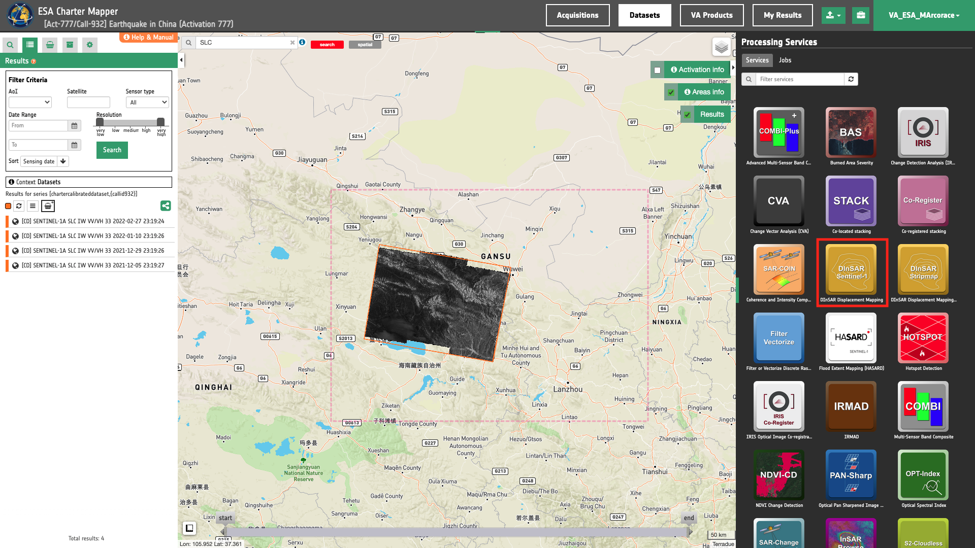
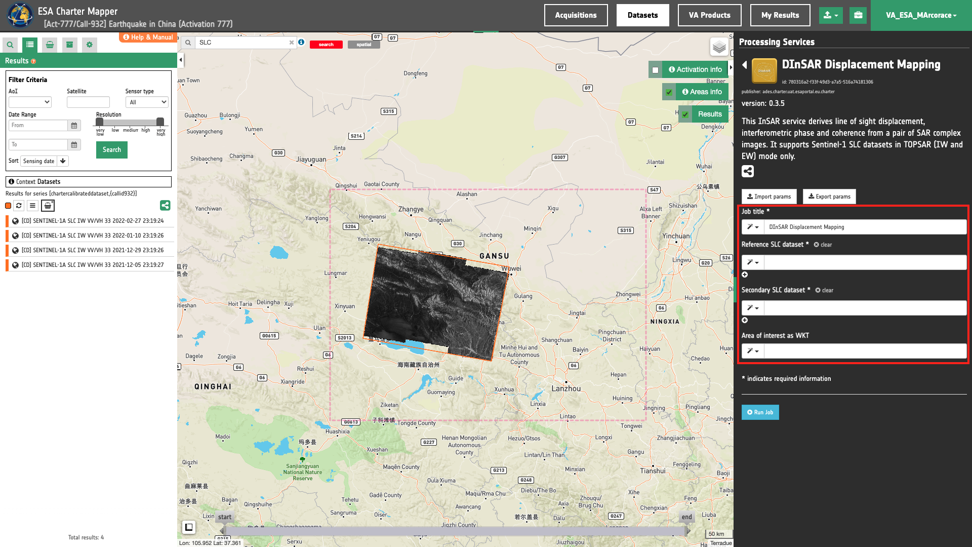
The "DInSAR Displacement Mapping - Sentinel-1 (DInSAR-S1)" panel is displayed with parameters values to be filled-in.
Find the data using multiple filter criteria
Choose an area in which you want to focus your analysis. As an example the Menyuan County, Qinghai Province near the border with Gansu Province, China.
From the Navigation and Search toolbar (located in the upper left side of the map), click on “Spatial Filter” and draw a square around your Area of Interest. This spatial filter allows you to select only the EO data acquired over this area.
From the top of the left panel, use Filter Criterias to search for Radar and sentinel-1 data collections from the list.
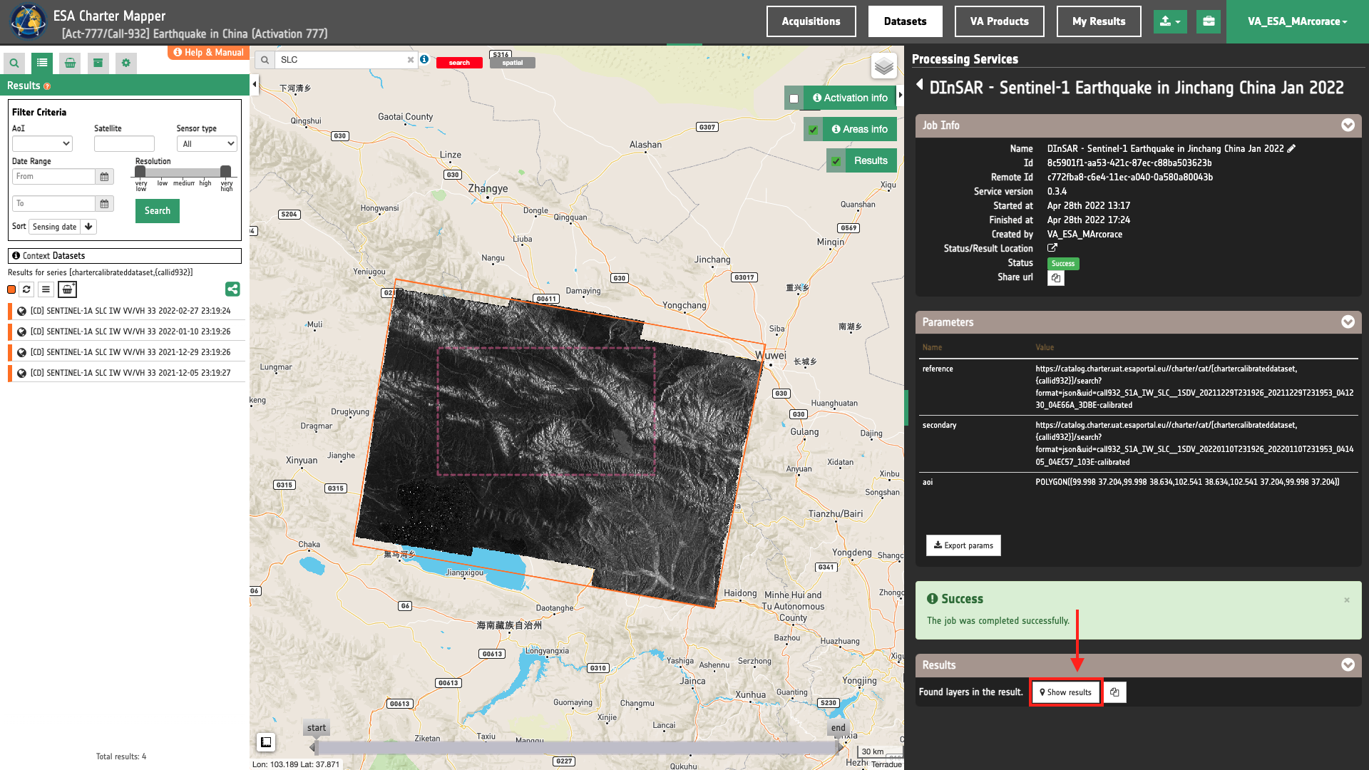
To further filter results by selecting only SLC products you can use the Text filter by inserting SLC in the Search Terms text box always visible on the top left of the map.
After the query, the Results list will include only the features satisfying all the above defined filters.
Now it is possible to choose a pair of "Reference" and "Secondary" SLC Datasets to be used for DInSAR. This pair must come from the same sensor and shall have the same radar geometry (incident angle, orbit path).
Fill the parameters
After the definition of all the filters, you can employ DInSAR by importing at least a pair of Sentinel-1 SLC Datasets.
Job name
Insert as job name:
DInSAR - Sentinel-1 Earthquake in Jinchang China Jan 2022
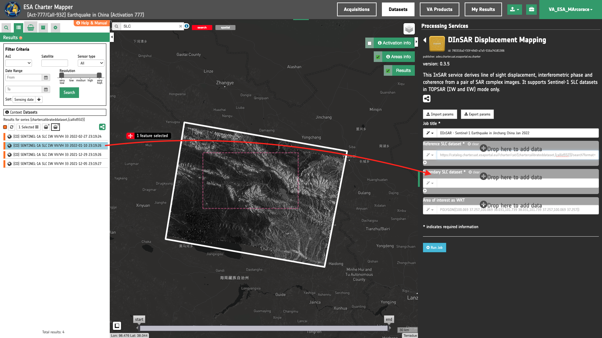
Input Reference and Secondary datasets
Drag and Drop in the Reference SLC dataset and in the Secondary SLC dataset fields the following datasets:
-
[CD] Sentinel-1A SLC VV/VH 33 29/12/2020 23:19:26,
-
[CD] Sentinel-1A SLC VV/VH 33 10/01/2021 23:19:26.
!! Tip For convention the reference is the oldest SAR acquisition and you can check how the motion was evolved by inserting the last acquired image as secondary.
Note
This service supports only SAR complex imagery.
Warning
DInSAR currently supports only SLC Datasets from the Sentinel-1 EO mission.
Warning
Drag and drop the Dataset (e.g. "[CD] Sentinel-1A SLC VV/VH 33 29/12/2020 23:19:26") and not the single-band asset (e.g. "magnitude-vh-iw1-001") into the Reference/Secondary SLC datasets fields.
Area of interest expressed as Well-known text
The “Area of interest as Well Known Text” can be defined by using the drawn polygon defined with the area filter.
Tip
In the definition of “Area of interest as Well Known Text” it is possible to apply as AOI the drawn polygon defined with the area filter. To do so, click on the button in the left side of the "Area of interest expressed as Well-known text" box and select the option AOI from the list. The platform will automatically fill the parameter value with the rectangular bounding box which is taken from the current search area in WKT format.
Note
This parameter is optional.
Once all parameters are inserted the processing service panel shall appear as the one shown in the figure below.
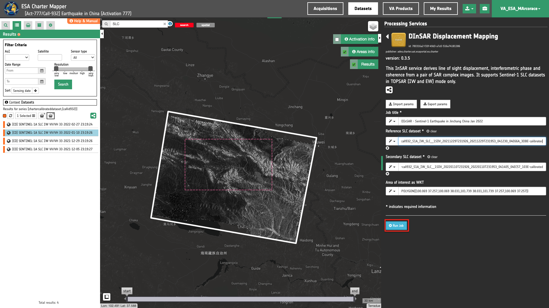
Run the job
Click on the button Run Job and see the Running Job. You can monitor job progress through the progress bar.
Results: download and visualization
Once the job is completed, click on the button Show results at the bottom of the processing service panel.
Tip
You can also save the parameters employed in this job by clicking on the Export params button in the right panel. This allows you to copy all your entries to the clipboard. This is meant to be used for a quick re-submission of a similar job after a fine tuning of the parameters (e.g. to add a colour formula later).
Below is reported the syntax which includes all the parameters employed in this example.
{
   "reference": "https://catalog.disasterscharter.org//charter/cat/[chartercalibrateddataset,{callid932}]/search?format=json&uid=call932_S1A_IW_SLC__1SDV_20211229T231926_20211229T231953_041230_04E66A_3DBE-calibrated",
   "secondary": "https://catalog.disasterscharter.org//charter/cat/[chartercalibrateddataset,{callid932}]/search?format=json&uid=call932_S1A_IW_SLC__1SDV_20220110T231926_20220110T231953_041405_04EC57_103E-calibrated",
   "aoi": "POLYGON((100.069 37.257,100.069 38.031,101.739 38.031,101.739 37.257,100.069 37.257))"
}
Visualization
See the result on the map. The preview appears within the area defined in the spatial filter.
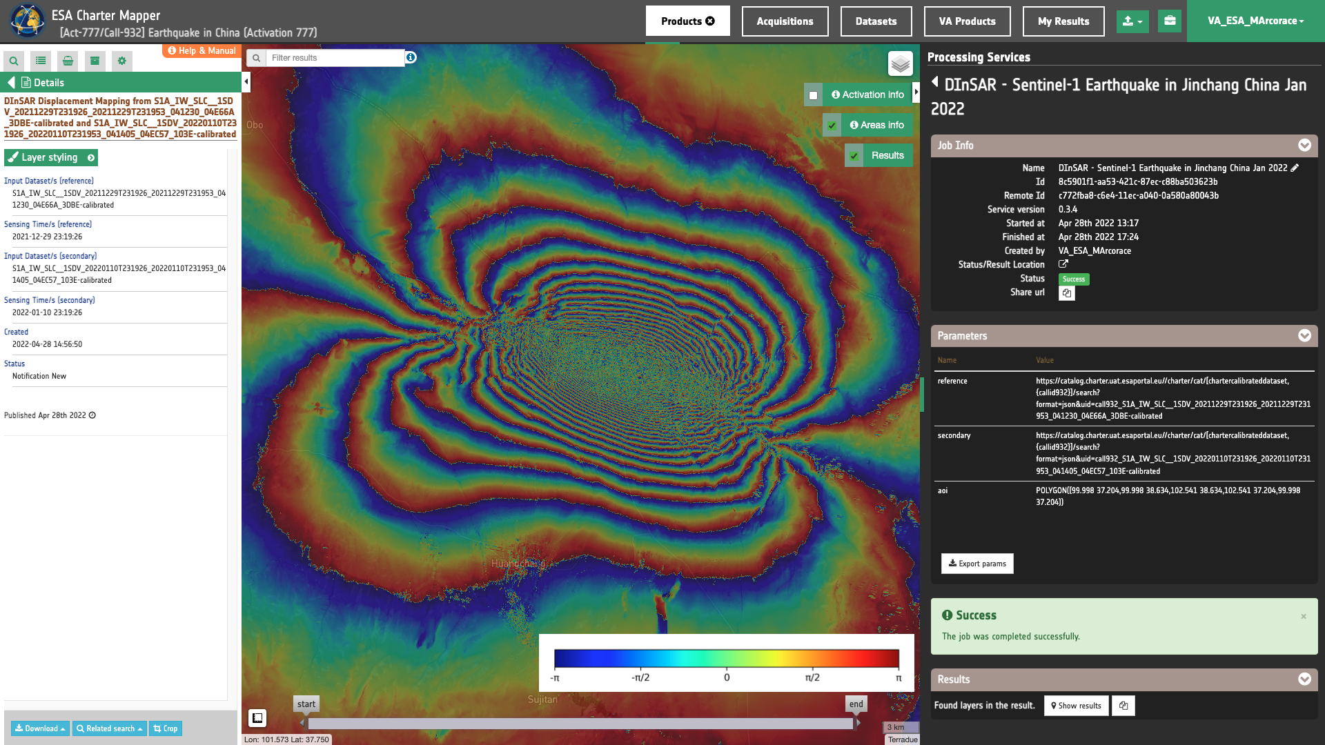
To get more information about the product just click on the preview in the map, a bubble showing the name of the layer “DInSAR Displacement Mapping from call932_S1A_IW_SLC__1SDV_20211229T231926_20211229T231953_041230_04E66A_3DBE-calibrated and call932_S1A_IW_SLC__1SDV_20220110T231926_20220110T231953_041405_04EC57_103E-calibrated” will appear and then click on the Show details button.
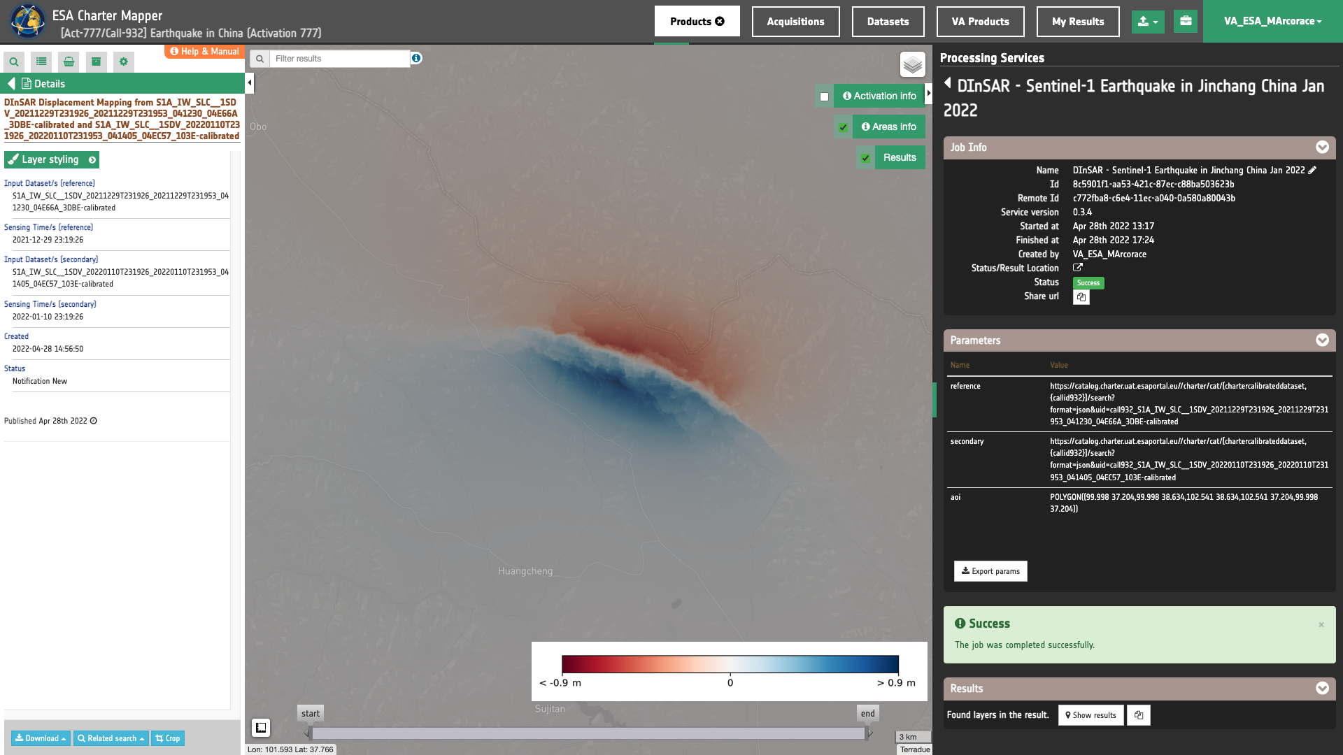
In the left panel under the result Details is possible to customize the overview on the fly by clicking on Layer Styling and Select Asset or Combine Assets. As an example under Select Assets you can select the asset displacement_c_vv_20211229_20220110 band change the color map and set the desired opacity level.
It is also possible to make RGB composites on the fly using the single band assets generated by the service. To do so click on Combine Assets and specify the assets in the RGB channels.
Warning
When combining single-band assets under Combine assets please consider the valid range associated with the specific asset. As an example consider [0,1] for coherence and [-3.14,3.14] for the interferometric phase in radians. Valid ranges for all single-band products can be found here. Min and Max values shall be inserted manually in the Channel histogram min/max boxes.
Download
In this first use case the DInSAR-S1 service returned as output the following 6 products:
- coh_c_vv_20210311_20210323: single-band asset
coh_c_vvproduct for Coherence in C-band and VV polarization from the interferometric pair 20211229_20220110 as single band GeoTIFF in COG format, - phase_c_vv_20210311_20210323: single-band asset
phase_c_vvproduct for the Interferometric Phase in C-band and VV polarization from the interferometric pair 20211229_20220110 as single band GeoTIFF in COG format, - displacement_c_vv_20210311_20210323: single-band asset
displacement_c_vvproduct for LOS displacement in C-band and VV polarization from the interferometric pair 20211229_20220110 as single band GeoTIFF in COG format. - overview-coherence: multi-band visual asset derived from the Interferometric Coherence product using the "Gray" color map given as 4-band 8-bit GeoTIFF in COG format,
- overview-phase: multi-band visual asset derived from the Interferometric Phase product in radians using the "Jet" color map given as 4-band 8-bit GeoTIFF in COG format,
- overview-displacement: multi-band visual asset derived from the Line of Sight Displacement in m product using a "RdBu" color map given as 4-band 8-bit GeoTIFF in COG format,
To download these products click on the Download button located at the bottom of the Product Details tab in the left panel. Users can also dowloand the legend of each overview asset in PNG format.
Use case 2: DInSAR with SAOCOM-1 data
Select the processing service
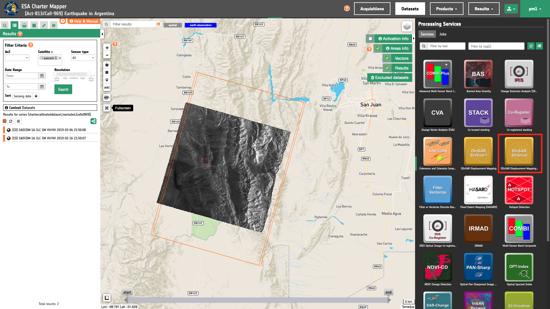
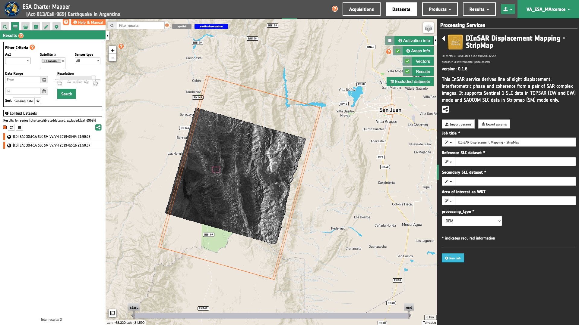
After the opening of the activation workspace, in the right panel of the interface, open the Processing Services tab and select the processing service DInSAR Displacement Mapping - Stripmap (DInSAR-SM).
The "DInSAR Displacement Mapping - Stripmap (DInSAR-SM)" panel is displayed with parameters values to be filled-in.
Find the data using multiple filter criteria
Choose an area in which you want to focus your analysis. As an example near San Juan in Argentina (EO data credits: CONAE)1.
From the Navigation and Search toolbar (located in the upper left side of the map), click on “Spatial Filter” and draw a square around your Area of Interest. This spatial filter allows you to select only the EO data acquired over this area.
From the top of the left panel, use Filter Criterias to search for Radar and saocom-1 data collections from the list.
To further filter results by selecting only SLC products you can use the Text filter by inserting SLC in the Search Terms text box always visible on the top left of the map.
After the query, the Results list will include only the features satisfying all the above defined filters.
Now it is possible to choose a pair of "Reference" and "Secondary" SLC Datasets to be used for DInSAR. This pair must come from the same sensor and shall have the same radar geometry (incident angle, orbit path).
Fill the parameters
After the definition of all the filters, you can employ DInSAR by importing at least a pair of Sentinel-1 SLC Datasets.
Job name
Insert as job name:
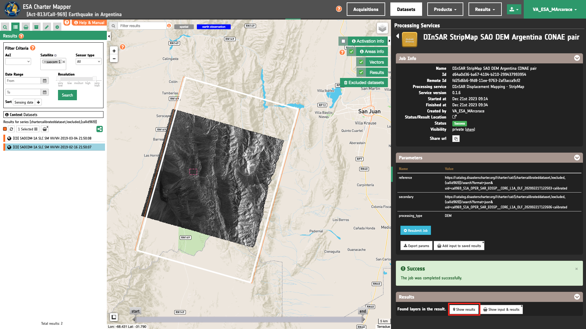
DInSAR Stripmap SAO DEM Argentina CONAE pair
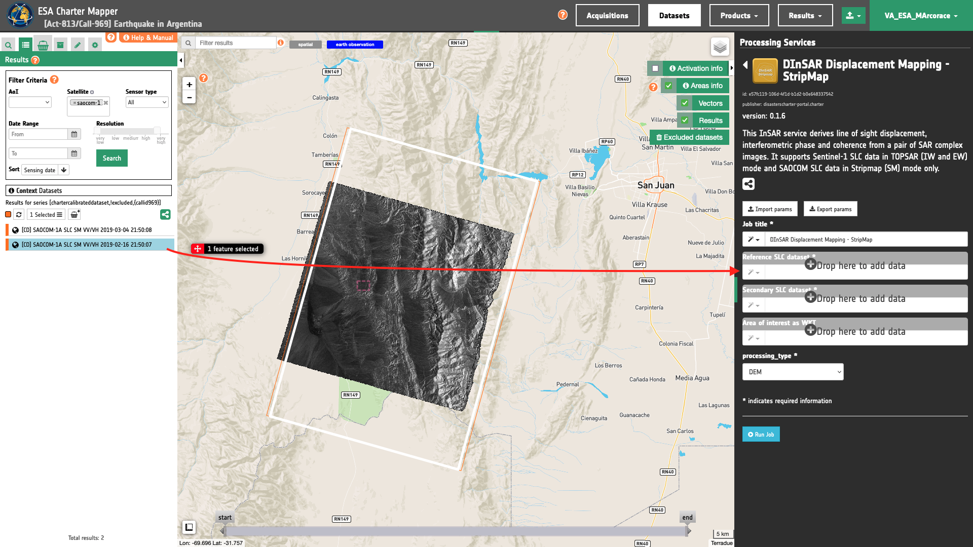
Input Reference and Secondary datasets
Drag and Drop in the Reference SLC dataset and in the Secondary SLC dataset fields the following datasets:
-
[CD] SAOCOM-1A SLC SM VV/VH 2019-03-04 21:50:08,
-
[CD] SAOCOM-1A SLC SM VV/VH 2019-02-16 21:50:07.
!! Tip For convention the reference is the oldest SAR acquisition and you can check how the motion was evolved by inserting the last acquired image as secondary.
Note
This service supports only SAR complex imagery.
Warning
DInSAR-SM currently supports only SLC Datasets in Stripmap mode from the Saocom-1 EO mission.
Warning
Drag and drop the Dataset (e.g. [CD] SAOCOM-1A SLC SM VV/VH 2019-03-04 21:50:08) and not the single-band asset (e.g. amplitude-vv) into the Reference/Secondary SLC datasets fields.
Processing type
With this parameter you shall choose among the 2 possible processing types for the generation of the interferogram:
-
DEM - a DEM assisted co-registration is employed for the interferogram generation,
-
XCORR - the interferogram is generated without the DEM through a sequence of stacking, cross-correlation, and warping of reference and secondary.
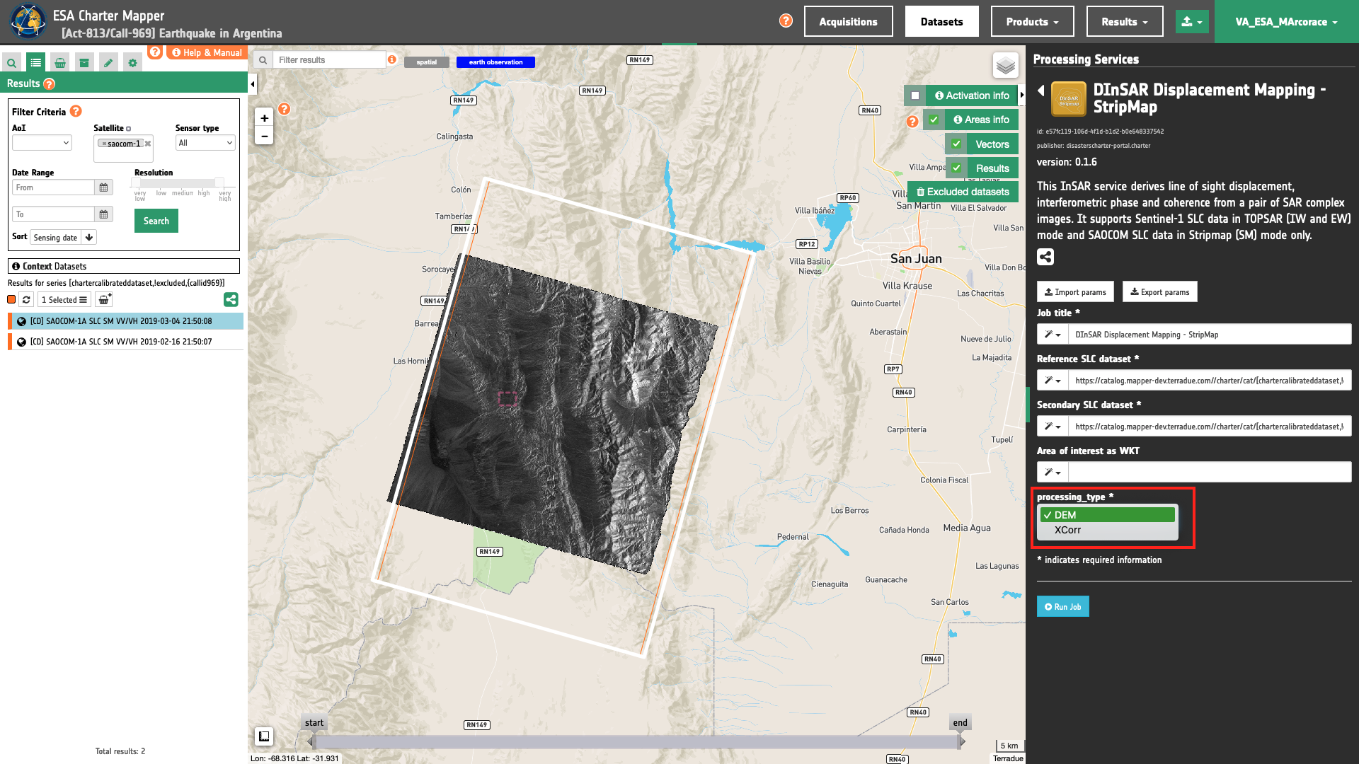
Leave the default option DEM.
Area of interest expressed as Well-known text
The “Area of interest as Well Known Text” can be defined by using the drawn polygon defined with the area filter.
Tip
In the definition of “Area of interest as Well Known Text” it is possible to apply as AOI the drawn polygon defined with the area filter. To do so, click on the button in the left side of the "Area of interest expressed as Well-known text" box and select the option AOI from the list. The platform will automatically fill the parameter value with the rectangular bounding box which is taken from the current search area in WKT format.
Note
This parameter is optional.
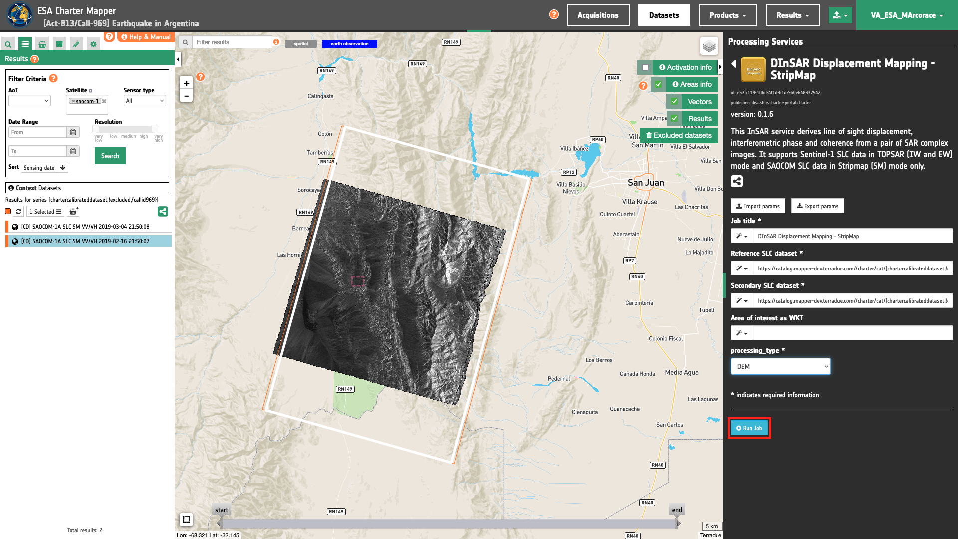
In this tutorial AOI is not defined.
Run the job
Once all parameters are inserted the processing service panel shall appear as the one shown in the figure below. Click on the button Run Job and see the Running Job. You can monitor job progress through the progress bar.
Results: download and visualization
Once the job is completed, click on the button Show results at the bottom of the processing service panel.
Tip
You can also save the parameters employed in this job by clicking on the Export params button in the right panel. This allows you to copy all your entries to the clipboard. This is meant to be used for a quick re-submission of a similar job after a fine tuning of the parameters (e.g. to add a colour formula later).
Below is reported the syntax which includes all the parameters employed in this example.
{
   "reference": "https://catalog.disasterscharter.org//charter/cat/[chartercalibrateddataset,!excluded,{callid969}]/search?format=json&uid=call969_S1A_OPER_SAR_EOSSP__CORE_L1A_OLF_20200221T122503-calibrated",
   "secondary": "https://catalog.disasterscharter.org//charter/cat/[chartercalibrateddataset,!excluded,{callid969}]/search?format=json&uid=call969_S1A_OPER_SAR_EOSSP__CORE_L1A_OLF_20200221T122606-calibrated",
   "processing_type": "DEM"
}
Visualization
See the result on the map. The preview appears within the area defined in the spatial filter.
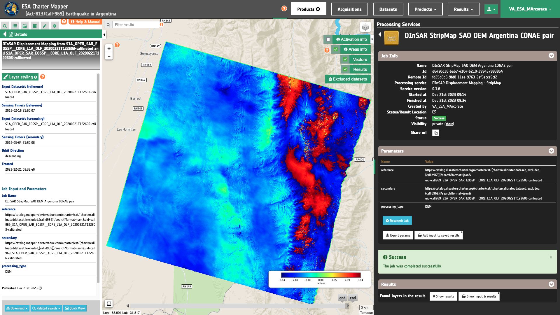
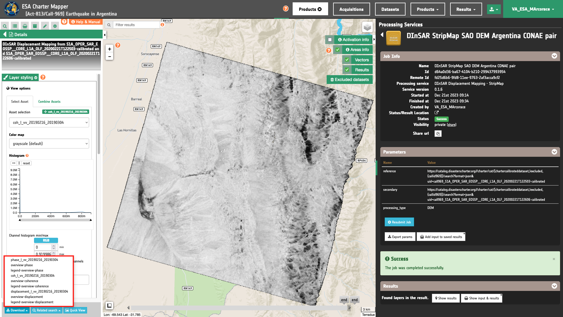
To get more information about the product just click on the preview in the map, a bubble showing the name of the layer “DInSAR Displacement Mapping from S1A_OPER_SAR_EOSSP__CORE_L1A_OLF_20200221T122503-calibrated and S1A_OPER_SAR_EOSSP__CORE_L1A_OLF_20200221T122606-calibrated” (Feature under the Results list with the tag DInSAR StripMap SAO DEM Argentina CONAE pair) will appear and then click on the Show details button.
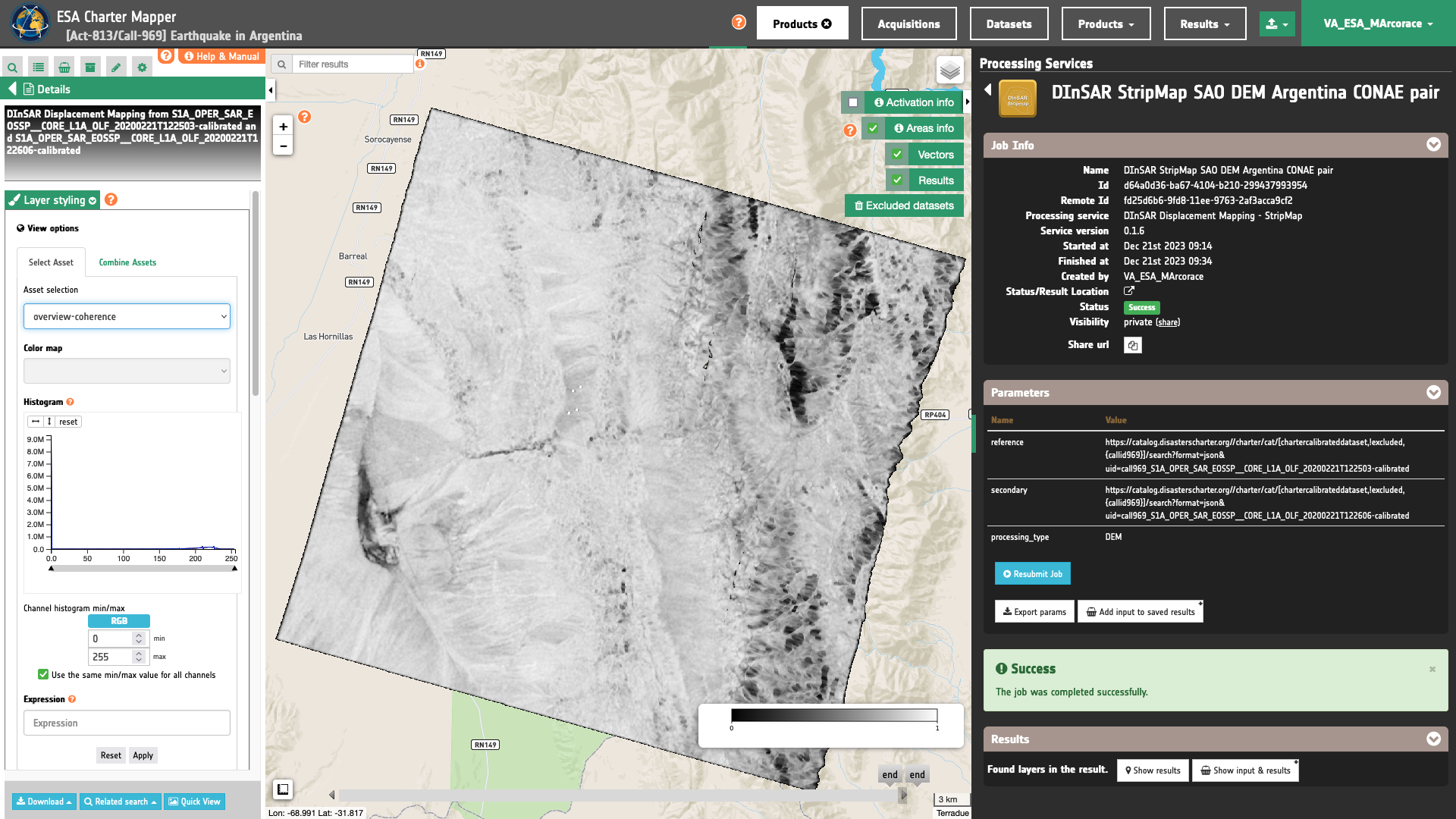
In the left panel under the result Details is possible to customize the overview on the fly by clicking on Layer Styling and Select Asset or Combine Assets. As an example under Select Assets you can select another asset, as the overview-coherence one, and visualize it in the geobrowser together with the legend displayed in the bottom righter corner of the map.
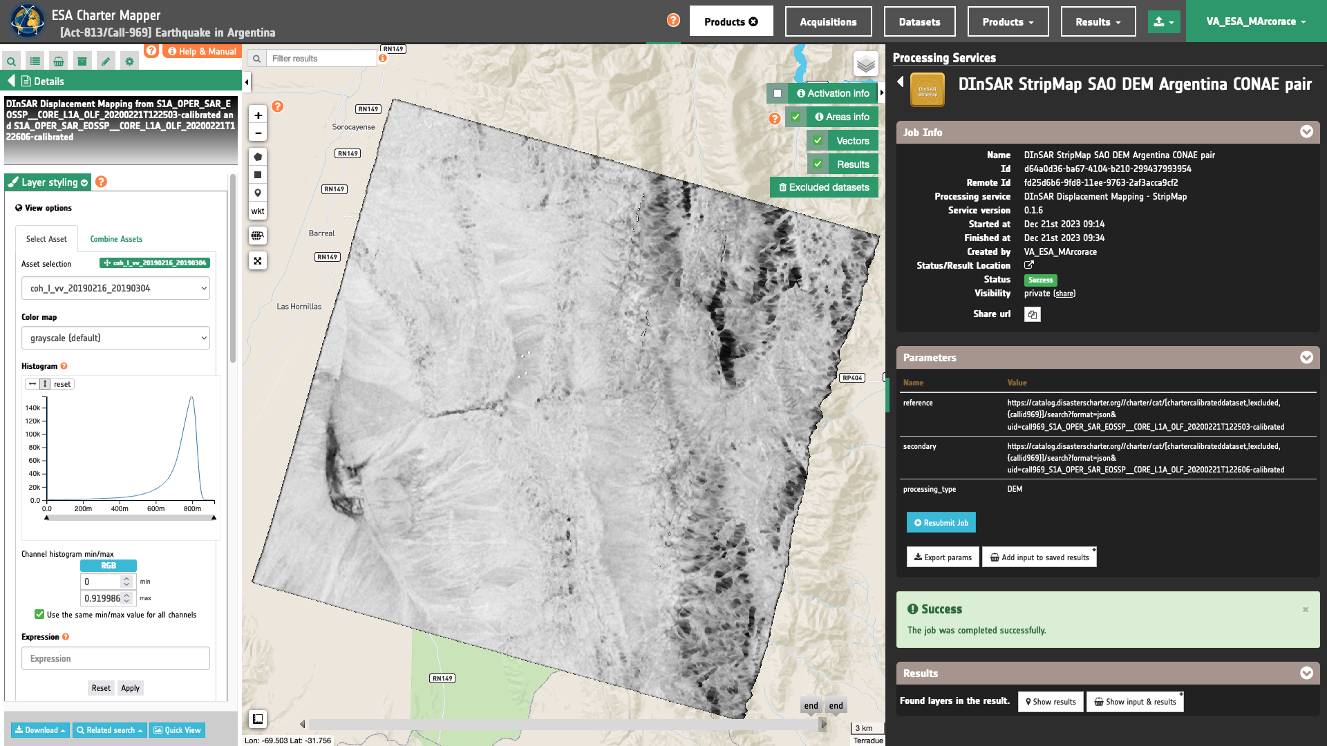
Same for a single band asset (e.g. by selecting coh_l_vv_20190216_20190304).
It is also possible to make RGB composites on the fly using the single band assets generated by the service. To do so click on Combine Assets and specify the assets in the RGB channels.
Warning
When combining single-band assets under Combine assets please consider the valid range associated with the specific asset. As an example consider [0,1] for coherence and [-3.14,3.14] for the interferometric phase in radians. Valid ranges for all single-band products can be found here. Min and Max values shall be inserted manually in the Channel histogram min/max boxes.
Download
In this second use case the DInSAR-SM service returned as output the following 6 products:
- coh_l_vv_20190216_20190304: single-band asset
coh_l_vvproduct for Coherence in L-band and VV polarization from the interferometric pair 20190216_20190304 as single band GeoTIFF in COG format, - phase_c_vv_20190216_20190304: single-band asset
phase_l_vvproduct for the Interferometric Phase in L-band and VV polarization from the interferometric pair 20190216_20190304 as single band GeoTIFF in COG format, - displacement_c_vv_20190216_20190304: single-band asset
displacement_l_vvproduct for LOS displacement in L-band and VV polarization from the interferometric pair 20190216_20190304 as single band GeoTIFF in COG format. - overview-coherence: multi-band visual asset derived from the Interferometric Coherence product using the "Gray" color map given as 4-band 8-bit GeoTIFF in COG format,
- overview-phase: multi-band visual asset derived from the Interferometric Phase product in radians using the "Jet" color map given as 4-band 8-bit GeoTIFF in COG format,
- overview-displacement: multi-band visual asset derived from the Line of Sight Displacement in m product using a "RdBu" color map given as 4-band 8-bit GeoTIFF in COG format,
To download these products click on the Download button located at the bottom of the Product Details tab in the left panel.
Users can also dowloand the legend of each overview asset in PNG format.
-
CONAE, SAOCOM 1A Test Products for satellite information users, Interferometric pair - Stripmap Dual Pol products, Area of El Leoncito National Park, San Juan Province, Argentina. Available at: https://catalogos.conae.gov.ar. ↩