STACK service specifications
![]()
This service provides a multi-mission and multi-temporal image stack of multiple co-located single-band assets against a reference one. The service supports single band assets taken from Optical or Radar Calibrated Datasets, Auxiliary Datasets or Results of other processors. It performs resampling and warping of secondary assets and the stacking of each secondary with the reference. It can also generate assets from the co-located stack using band arithmetic.
 The tutorial of the STACK service is available in this section.
Service Description
The Co-located Stacking (STACK) service computes the co-location of single-band assets having different map projections and spatial resolutions on a common grid. It performs resampling and warping of the secondary assets and the stacking of each secondary with the reference. The upsampling or/and downsampling of spatially overlapping assets is performed on a common area (intersection based on STAC asset geometry) and is based only on pixel coordinates. The service requires input geocoded assets, which are a prerequisite for the stacking service. As an example, input single-band assets can be taken from multi-sensor Optical or SAR Calibrated Datasets, Results of other on-demand processing services, and Auxiliary Datasets. For more details find the section about inputs here. It can also generate assets from the co-located stack using band arithmetic (via s-expressions). Co-location results depend on the level of accuracy of geopositioning of source images. The Co-located Stacking processor is built with the GDAL VRT method1. It can also generate new assets from the co-located stack using band arithmetic with symbolic expression (S-expression).
Workflow
The service implements the workflow depicted below.
Input
Input of the STACK service can be geocoded images from supported SAR or optical sensors (e.g. reflectance or Sigma Nought single-band assets from Calibrated Datasets derived systematically in the calibration processing from supported Optical or SAR sensors). Co-location stacking is also possible if the input set of images is built by mixing single band assets from SAR and Optical Calibrated Datasets. Also, input single band assets in STACK can originates from Results of some on-demand processing services and from Auxiliary Datasets.
STACK supports single-band assets derived from the following services: PAN-Sharp, OPT-Index, BAS, IRIS, HOTSPOT, HASARD Dual Image, and the two InSAR processors DInSAR, and SAR-COIN (for coherence asset only).
It also supports single band assets from the following Auxiliary Datasets:
-
HAND.
Parameters
The STACK service requires a specified number of mandatory and optional parameters. All service parameters are listed in the below Table 1.
| Parameter | Description | Required | Default value |
|---|---|---|---|
| Single band asset(s) | List of single band assets to be colocated from Datasets, Aux Datasets or Results of processors | YES | |
| Area of Interest | Area of interest expressed in WKT | NO | |
| S-expression/s | S-expression/s to generate additional asset/s from the ones in the stack (e.g. average) | NO |
Table 1 - Service parameters for the STACK processor.
More information about the service parameters are given below.
Input single band assets
This first mandatory parameter is the list of input single band assets that are used to create the collocated stack. These assets can originate from:
-
Optical or Radar Calibrated Datasets,
-
Auxiliary datasets,
-
Results from on-demand processing (e.g. from HASARD Dual Image, or SAR-COIN).
Inputs are the path to the single band assets from the chosen Calibrated Datasets, Aux Dataset, or Results STAC items.
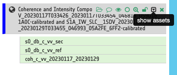
In the definition of each input single band asset the drag and drop of single-band asset/s is foreseen. This is possible by dragging and dropping one of the single-band assets included into a Calibrated Dataset, Aux Dataset or Results. These assets can be easily retrieved by showing the single band assets of a Dataset, Aux Dataset or Result features in the Results panel or in the features basket.
Hint
To find the single band assets of a Calibrated Dataset, click on the Show assets button available near the feature title. A list with all single-band assets (CBNs) included within the Calibrated Dataset will appear under the feature title.
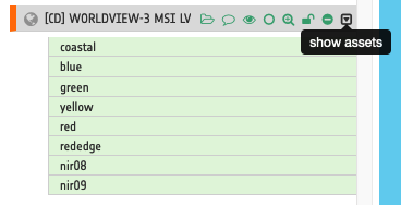
Same to find single band assets from Aux Datasets, or Results of on-demand processing.
The drag and drop of the single band asset (e.g. nir) provides to the service a string in the format
input_dataset#single-band_asset
As an example, after the drag and drop the following string will be automatically inserted as a value for the parameter:
https://catalog.disasterscharter.org//charter/cat/[chartercalibrateddataset,{callid895}]/search?format=json&uid=call895_PT01N07_966794E007_8043502022080500000000MS00_GG003002001-calibrated#nir"
If multiple selected single band assets (e.g. red, nir) from a single dataset are defined via a single drag and drop interaction the string becomes:
input_dataset#asset1,asset2,assetN
As an example, after the drag and drop the following string will be automatically inserted as a value for the parameter:
https://catalog.disasterscharter.org//charter/cat/[chartercalibrateddataset,{callid895}]/search?format=json&uid=call895_PT01N07_966794E007_8043502022080500000000MS00_GG003002001-calibrated#red,nir"
Hint
Use CONTROL + click to select more than an asset from the list.
In this way the STACK processor is able to get the path to the single band assets from the chosen Calibrated Datasets, Aux Dataset, or Results STAC items.
Note
This string format is the only type of input accepted.
Warning
Users must drag and drop the single-band asset (e.g. nir for reflectance or s0_db_c_vv for backscatter in VV polarization and C-band) into the Input single band asset(s) parameter. The drag and drop of the Calibrated Dataset (e.g. "[CD] PLANETSCOPE PSB.SD L3B 2022-08-05 09:01:35") is not enough.
Note
The specified input single band asset must be at least one single-band asset.
Warning
In the co-location only single-band assets can be used (e.g. reflectance, backscatter, binary change mask or coherence) and not overview ones.
AOI (optional)
This second parameter (optional) may define the area of interest expressed as a Well-Known Text value.
Warning
If set, it overrides the automatic determination of the maximum common area between the geometry of each input single band asset.
Tip
In the definition of “Area of interest as Well Known Text” it is possible to apply as AOI the drawn polygon defined with the area filter. To do so, click on the Magic tool wizard button in the left side of the "Area of interest expressed as Well-known text" box and select the option AOI from the list. The platform will automatically fill the parameter value with the rectangular bounding box taken from the current search area in WKT format.
S-expression (optional)
This third optional parameter allows generating new single-band assets derived from the collocated image stack (e.g. average, normalized difference etc.) using band arithmetic with symbolic expressions (S-expression).
How to specify input assets in symbolic expressions
After the drag and drop the STACK creates an indexing of all single band assets based on a prefix with the number of source Datasets or Result (1 for first dataset, 2 for the second one, etc.). Thus, to employ a single band asset in band arithmetic with STACK the user shall specify it as following:
dataset_or_result_number.single-band_asset
Note
This syntax is important to correctly employ a single band asset in the band arithmetic of STACK with s-expressions.
Tip
Always check the list of CBNs available in a Calibrated Dataset (or the name of single band assets included into an Auxiliary Dataset or a Result of a processing service) after the drag and drop as well as before specifying a single-band asset in a symbolic expression. A Worldview-2 MS Calibrated Dataset does not have a nir asset but a nir08 one. The ESA World Cover Auxiliary Dataset has only one single-band asset named worldcover. Results from similar on-demand change detection processing services may have multiple single-band assets with different STAC keys (e.g. flood-mask for HASARD Dual Image and cva_change_detection for CVA).
Note
All CBNs available in the ESA Charter Mapper can be found here.
Example
To build a STACK using multiple reflectance single band assets (e.g. coastal, blue, green, red, and nir) from a single Calibrated Dataset the users shall drag and drop 5 input reflectance single band assets in STACK from the same Dataset. In total dragging and dropping 5 assets in the first STACK parameter.
Being the 5 assets originated from a single Dataset the prefix of each assets is 1 and in band arithmetic each asset shall be defined as:
- 1.coastal
- 1.blue
- 1.green
- 1.red
- 1.nir
Example
To build a multitemporal STACK using multiple backscatter single band assets (e.g. s0_db_c_vv, and s0_db_c_vh) from three Calibrated Datasets the users shall drag and drop 2 input backscatter single band assets in STACK from 3 Datasets. In total dragging and dropping 6 assets in the first STACK parameter.
Being the 6 input assets originated from 3 different Radar Calibrated Datasets the prefix of each assets will be 1, 2, or 3 according to the order in which the assets are specified in input. Thus when employing these single band assets in band arithmetic each of them shall be defined as:
- 1.s0_db_c_vv
- 1.s0_db_c_vh
- 2.s0_db_c_vv
- 2.s0_db_c_vh
- 3.s0_db_c_vv
- 3.s0_db_c_vh
Example
To build a co-located stack using a pair of two coherence single band assets (e.g. coh_c_vv_20220330_20220411,, and coh_c_vv_20220517_20220529) derived from two SAR-COIN Result, obtained by exploiting 4 Sentinel-1 SLC Datasets acquired on 20220330, 20220411, 20220517, and 20220529 the user shall drag and drop 1 input coherence single band assets in STACK from 2 SAR-COIN Results. In total dragging and dropping 2 assets in the first STACK parameter.
Being the 2 input assets originated from 2 different SAR-COIN Results the prefix of each assets will be 1, or 2 according to the order in which the assets are specified in input. Thus when employing these single band assets in band arithmetic each of them shall be defined as:
- 1.coh_c_vv_20220330_20220411
- 2.coh_c_vv_20220517_20220529
Example
It is also possible to build a co-located stack by mixing different types of single-band assets derived from Results of other processing services. As an example to co-locate the flood-mask single band asset from HASARD Dual Image, and the cva_change_detection one from CVA, the user can first drag and drop 1 input flood mask single band asset from 1 HASARD Dual Image Result and then 1 input change detection mask single band asset from 1 CVA Result. In total dragging and dropping 2 assets in the first STACK parameter.
Being the 2 input assets originated from 2 Results of different processors the prefix of each assets will be 1, or 2 according to the order in which the assets are specified in input. Thus when employing these single band assets in band arithmetic each of them shall be defined as:
- 1.flood-mask
- 2.cva_change_detection
Example
Co-located stacking also supports single-band assets from Auxiliary Datasets. As an example to co-locate the flood-mask asset from HASARD Dual Image, and the worldcover one from ESA World Cover Auxiliary Dataset, the user can first drag and drop 1 input flood mask single band asset from 1 HASARD Dual Image Result and then 1 input land cover single band asset from 1 ESA World Cover Auxiliary Dataset. In total dragging and dropping 2 assets in the first STACK parameter.
Being the 2 input assets originated from 2 different sources (a Result from on demand processing and an Auxiliary Dataset) the prefix of each assets will be 1, or 2 according to the order in which the assets are specified in input. Thus when employing these single band assets in band arithmetic each of them shall be defined as:
- 1.flood-mask
- 2.worldcover
How to define a symbolic expression
In STACK band arithmetic, a new asset is defined with the name of the new output asset and it's associated s-expression separated by a colon : .
output_asset_name:(s-expression)
Warning
S-expressions can be made by using only the assets specified in input via the drag and drop and not with all the assets available in the source Dataset, Aux Dataset or Result.
Warning
The s-expressions inserted by the user must be given within brackets.
As an example to derive a new asset as the average between red bands from a pair of input single band assets (1.red and 2.red):
average:(/ (+ 1.red 2.red) 2)
This will add a new asset called average in the co-located stack with average values derived from 1.red and 2.red.
Arithmetic/logical operators and functions
S-expressions in the ESA Charter Mapper supports arithmetic (* + / -) and logical (< <= == != >= > & |) operators plus some pre-defined functions.
More information about supported functions can be found in Table 2.
| Function | Description | Syntax |
|---|---|---|
| asarray | convert the input (list, tuples, etc.) to an array | (asarray x) |
| interp | returns the one-dimensional piecewise linear interpolant to a function with given discrete data points (xp, fp), evaluated at x | (interp x xp fp) |
| mean | returns the mean value (scalar) from the given input array x | (mean x) |
| norm_diff | returns the normalized difference between A and B as per ((x - y) / (x + y)) | (norm_diff x y) |
| where | return elements chosen from x or y depending on condition | (where (condition) x y) |
Table 2 - Supported functions that can be used in s-expressions.
Note
The current list of functions can be further expanded in the future based on the user needs.
Examples of s-expressions which can be used to generate new bands from the STACK are listed in the below sections.
Compute sum
The following s-expression:
sum:(+ 1.pan 2.pan)
can be used to generate a band as the sum of 1.pan and 2.pan.
Compute difference
The following s-expression:
difference:(- 1.pan 2.pan)
can be used to generate a band as the difference of 1.pan and 2.pan.
Compute average
The following s-expression:
average:(/ (+ 1.pan 2.pan) 2)
can be used to generate a band as the average between the values of 1.pan and 2.pan.
Compute difference from average
The following s-expression:
diff_from_avg:(- 1.pan (mean 1.pan))
can be used to estimate a band of difference from the average value of 1.pan.
Compute normalized difference
The following s-expression:
ndvi:(norm_diff 1.nir 1.red)
can be used to derive multiple spectral indexes defined as normalized difference (e.g. NDVI, NDWI, NDBI, etc.).
Interpolate or rescale
The following s-expression:
rescaled:(interp 1.red (asarray 0 10000) (asarray 0 1))
can be used to interpolate the rescaled TOA reflectance into its original [0,1] range. Here (asarray 0 10000) returns [0, 10000] and is used to specify input range to be used for the interpolation.
Binarization
The following s-expression:
opt_water_mask:(where (>= (norm_diff 1.green 1.nir) 0.3) 1 0)
can be used to derive a water mask from the binarization of a spectral index. Here (norm_diff 1.green 1.nir) is used to derive the NDWI index. The value 0.3 represents the threshold as TOA reflectance. Similar s-expressions can be made also for SAR such as:
sar_water_mask:(where (<= 1.s0_db_c_hh -23) 1 0)
in which 1.s0_db_c_hh is the asset and the value -23 represents the threshold as Sigma Nought in dB.
Combine Datasets, Results and Auxiliary Datasets
STACK can be used also to post-process an asset from a Result of another processor. For instance, this makes it possible to co-locate a binary flood map from the Result of the HASARD Dual Image on-demand service with the Land Cover Auxiliary Dataset to extract flooded pixels over only a certain LC class. As an example the following s-expression:
flooded_cropland:(where (== 2.worldcover 40) 1.flood-mask 0)
can be used to derive a flood mask over only crop fields. In this case the s-expression (where (== 2.worldcover 40) 1.flood-mask 0)) is used to generate the flooded_cropland asset from the flood-mask one using the condition (== 2.worldcover 40). The value 40 represents the pixel value of the LC class cropland for the single-band asset worldcover offered in the ESA World Cover Auxiliary Dataset.
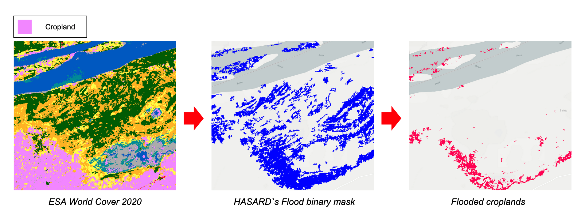
Figure 1 - Extraction of flooded cropland using the STACK service from a co-location of an HASARD-DI`s binary flood map and the ESA world Cover.
Hint
Specifications of the worldcover single band asset can be found here.
Output
The output of STACK is a multi-mission and multitemporal co-located stack with N single band assets in COG format. The output STAC item includes as many assets as provided in input plus the ones generated with s-expressions.
STACK Product specifications can be found in the table below.
| Attribute | Value / description |
|---|---|
| Long Name | Co-located stack from Optical or SAR EO data |
| Short Name | source_reference_number.source_asset (e.g. 1.nir) |
| Description | Multiband co-located stack of N images from optical and radar sensors |
| Processing level | L1 / L2 (according to input) |
| Data Type | Float32 |
| Band | N single-band |
| Format | COG |
| Projection | According to input |
| Fill Value | According to input |
-
GDAL documentation, gdalbuildvrt, available at: https://gdal.org/programs/gdalbuildvrt.html. ↩