STACK tutorial
![]()
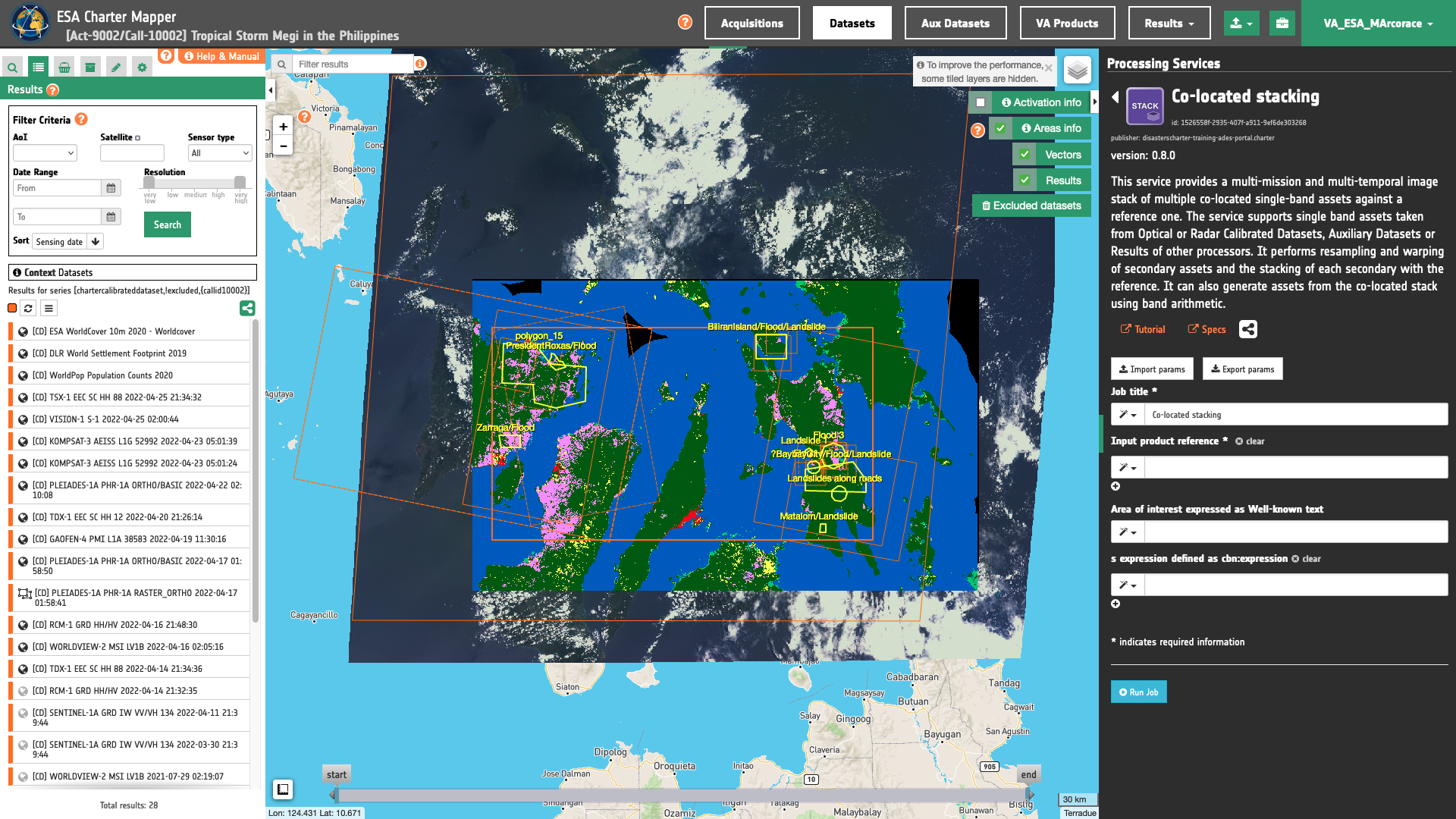
This service provides a multi-mission and multi-temporal image stack of multiple co-located single-band assets against a reference one. The service supports single band assets taken from Optical or Radar Calibrated Datasets, Auxiliary Datasets or Results of other processors. It performs resampling and warping of secondary assets and the stacking of each secondary with the reference. It can also generate assets from the co-located stack using band arithmetic.
 STACK service description and specifications are available in this section.
Select the processing service
After the opening of the activation workspace, in the right panel of the interface, open the Processing Services tab and select the processing service Co-located stacking (STACK).
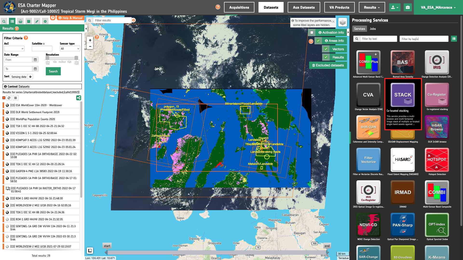
The Co-located stacking (STACK) panel is displayed in the right panel of the interface with a series of parameters values to be filled-in.
Hint
To easily find the STACK service in the list under the Services tab, employ the Filter by tag(s) function by selecting the ImageStack tag.
Note
A description of the Filter by tag(s) function can be found here.
Use cases
STACK is an advanced processing service that does not only perform a co-location of multi-sensor single band assets, but thanks to its band arithmetic function it can be used for multiple applications. Below are listed some possible use cases:
-
Generate NDVI change red-cyan composite from a co-located stack of pre- and post-event reflectance assets derived from different sensors,
-
Generate a multi-temporal co-located stack of images from the same sensor using SAR EO data and generate water masks,
-
Generate coherence loss map from a co-located stack of pre- and post-event coherence assets derived from the same sensor.
Use case 1: evaluate NDVI changes from a co-located stack of pre- and post-event images from different sensors
Abstract
This first use case explains how to create a stack of co-located images and derive from it pre- and post-event NDVI (Rouse et al., 1973)[^1] spectral indexes for a preliminary delineation of a landslide.
Find the data using multiple filter criteria
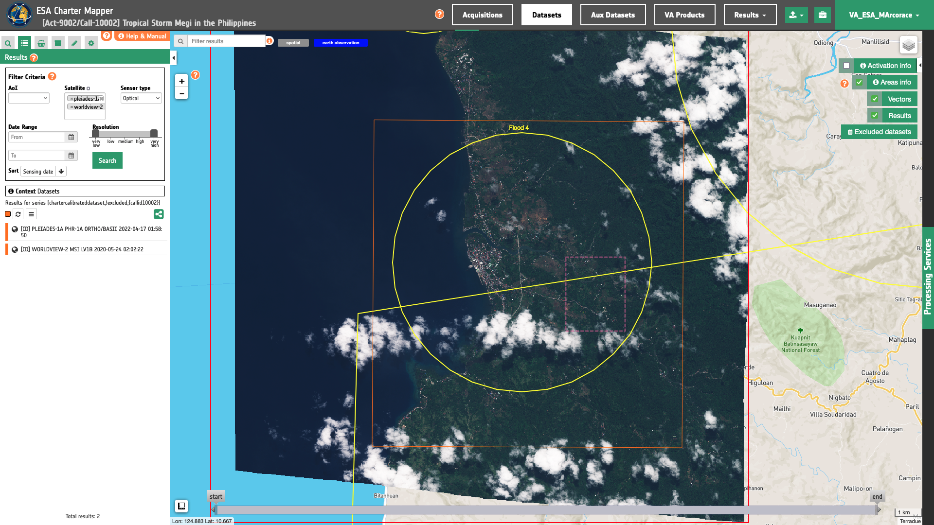
Choose an area in which you want to focus your analysis (e.g in Baybay, Philippines).
From the Navigation and Search toolbar (located in the upper left side of the map), click on “Spatial Filter” and draw a square around the north western of Baybay municipality. This spatial filter allows you to select only the EO data acquired over this area.
From the top of the left panel, use Filter Criteria to search for Pleiades-1a, and Worldview-2 data collections.
Once these filters are in place the Result list is updated as shown in the below figure.
Fill the parameters
After the definition of spatial and time filters, you can apply the co-located stacking, by importing, for example, two single-band assets from two calibrated datasets (in total 4 assets), as an example:
-
redandnir08assets from the Worldview-2 pre-event calibrated dataset -
and
redandnirassets from the Pleiades-1 post-event calibrated Datasets.
In this example the first input calibrated dataset is the Worldview-2 MSI L1B [CD] acquired on 24/05/2020, the second one is the Pleiades-1A MS ORTHO [CD] acquired on 17/04/2022.
Job name
Insert as job name:
STACK - NDVI change - Landslide in Baybay Philippines Apr 2022
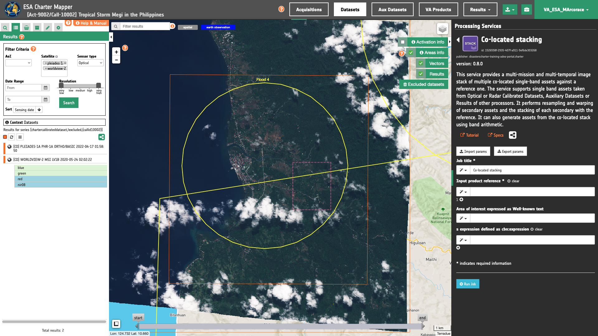
Input single band assets
To create NDVI from 2 calibrated datasets acquired from 2 different EO missions before and after an event the red and nir (or nir08) reflectance single-band assets are needed to make a co-location in STACK. Drag and Drop in the "Input single band asset(s)” field the red and nir (or nir08) single band assets from the following calibrated datasets:
-
[CD] WORLDVIEW-2 MSI LV1B 2020-05-24 02:02:22,
-
[CD] PLEIADES-1A PHR-1A ORTHO/BASIC 2022-04-17 01:58:50.
To do so, move the cursor over the first feature under the Results list, WORLDVIEW-2 MSI LV1B 2020-05-24 02:02:22. Features button will appear over the feture title. Click on the Show Assets button to reveal the list of single band assets contained in the Calibrated Dataset. Select red and nir08.
Hint
Use CONTROL + click to select more than an asset from the list.
Once the two assets from the first dataset are selected, drag and drop them into the Input single band asset(s) field. A string will be automatically inserted as first value for the first STACK parameter.
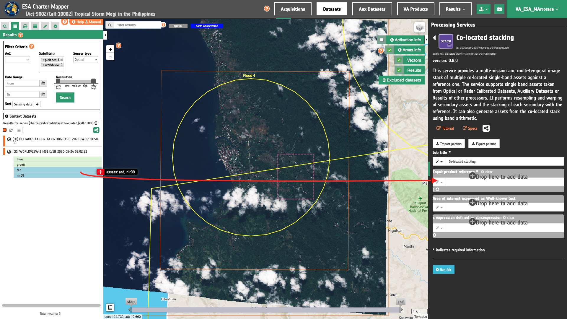
Repeat the drag and drop for the other 2 single band assets from the second dataset.

Being the 4 input assets originated from 2 different Optical Calibrated Datasets the prefix of each pair of assets will be 1, or 2 according to the order in which they are specified in input.
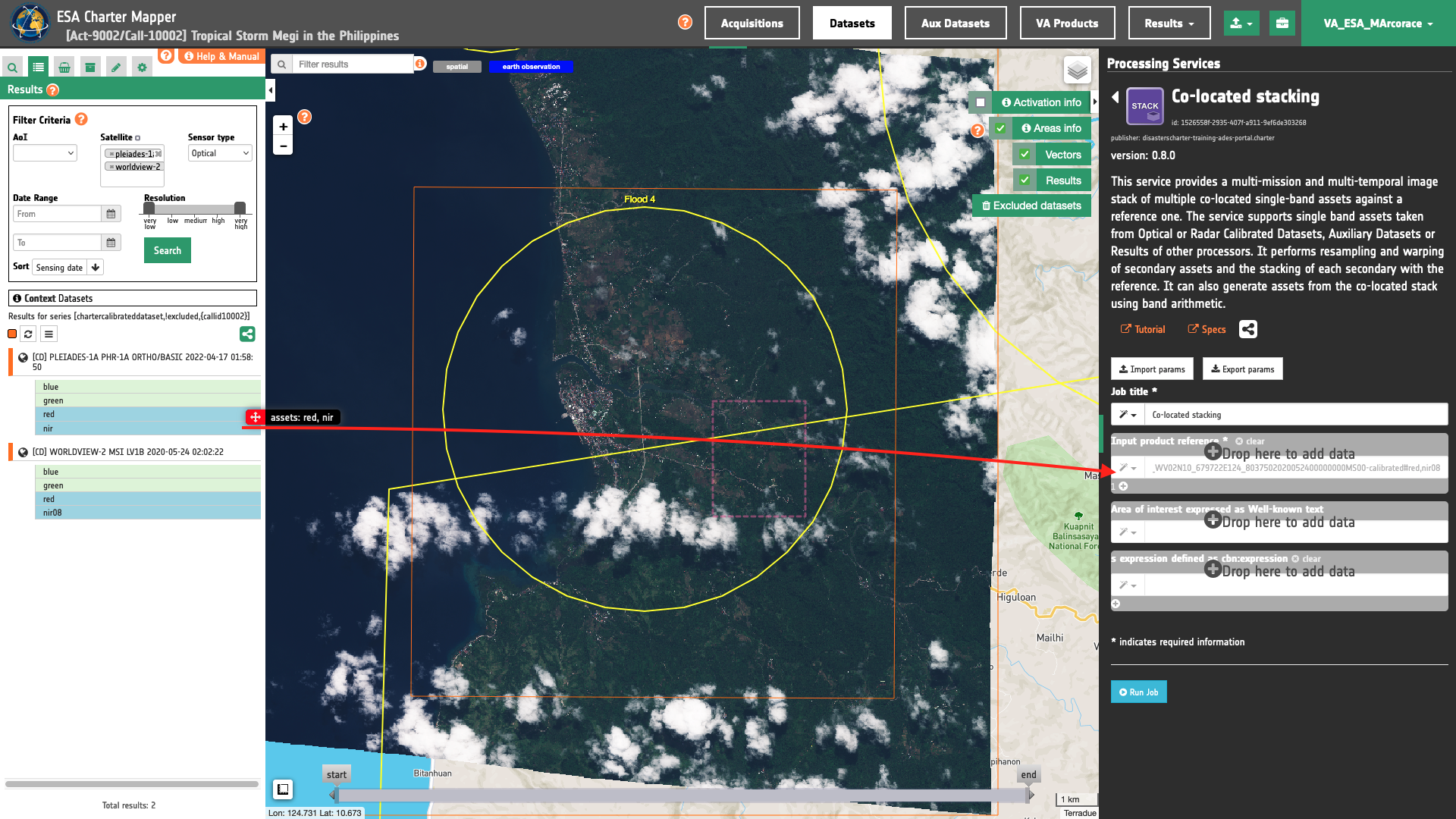
Thus when employing these single band assets in band arithmetic each of them shall be defined as:
-
1.red -
1.nir08 -
2.red -
2.nir
Tip
Always check the list of CBNs available in a Calibrated Dataset when dragging and dropping the single-band assets. A Worldview-2 MS Calibrated Dataset does not have a nir asset but a nir08 one.
Note
All CBNs available in the ESA Charter Mapper can be found here.
Warning
Drag and drop the single-band asset (e.g. "red") and not the Dataset (e.g. "[CD] PLEIADES-1B PHR-1B ORTHO/BASIC 2021/09/30 04:07:39") into the Input single band asset(s) field.
Area of interest expressed as Well-known text
The “Area of interest as Well Known Text” can be defined by using the drawn polygon defined with the area filter.
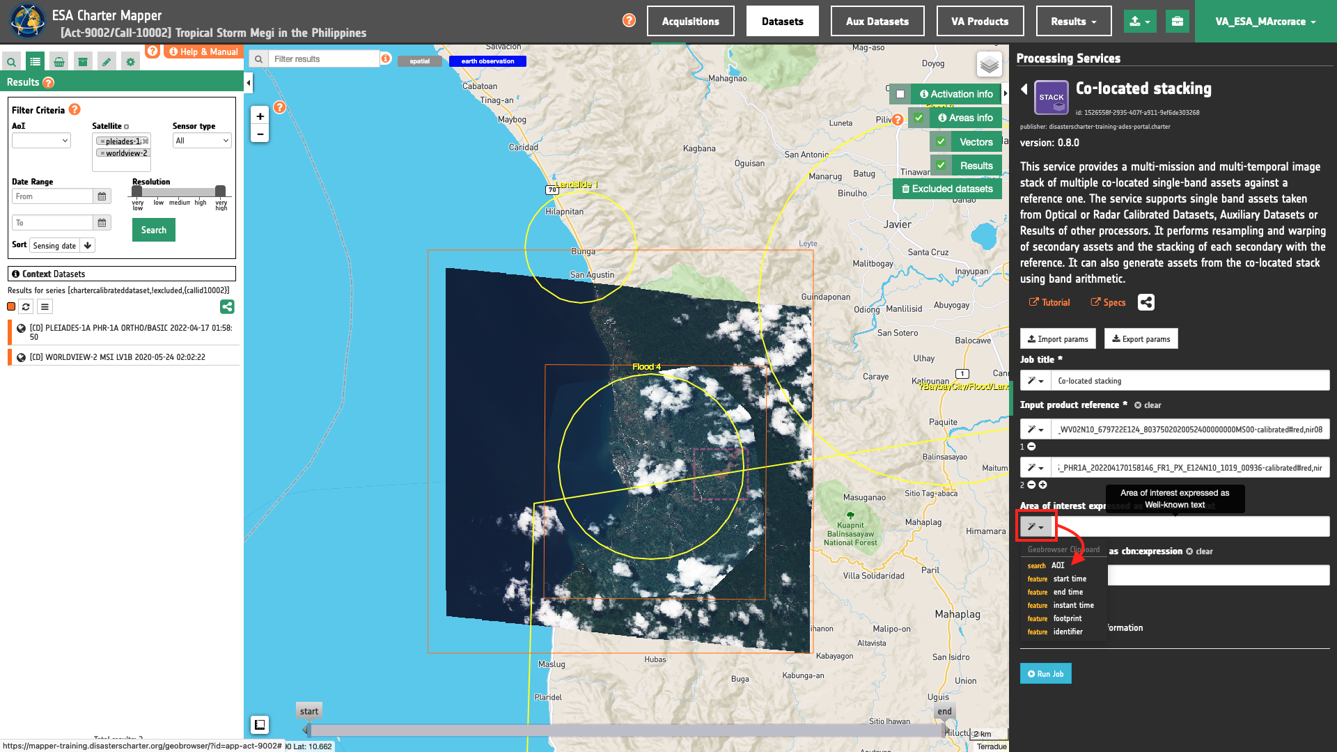
Tip
In the definition of “Area of interest as Well Known Text” it is possible to apply as AOI the drawn polygon defined with the area filter. To do so, click on the button in the left side of the "Area of interest expressed as Well-known text" box and select the option AOI from the list. The platform will automatically fill the parameter value with the rectangular bounding box which is taken from the current search area in WKT format.
Note
This parameter is optional.
S-expression
The remaining optional parameter to be filled in is the one dedicated for generating new bands from the ones present in the stack using s-expressions. In STACK a new band generated from the image stack is defined with a band name and it's associated s-expression separated by a colon : .
output_band_name:(s-expression)
To generate NDVI spectral indexes from pre- and post-event red and nir (or nir08) single band assets, insert the following s-expressions to generate four new bands in the image stack using the six input multispectral ones:
ndvi_pre:(norm_diff 1.nir08 1.red)
ndvi_post:(norm_diff 2.nir 2.red)
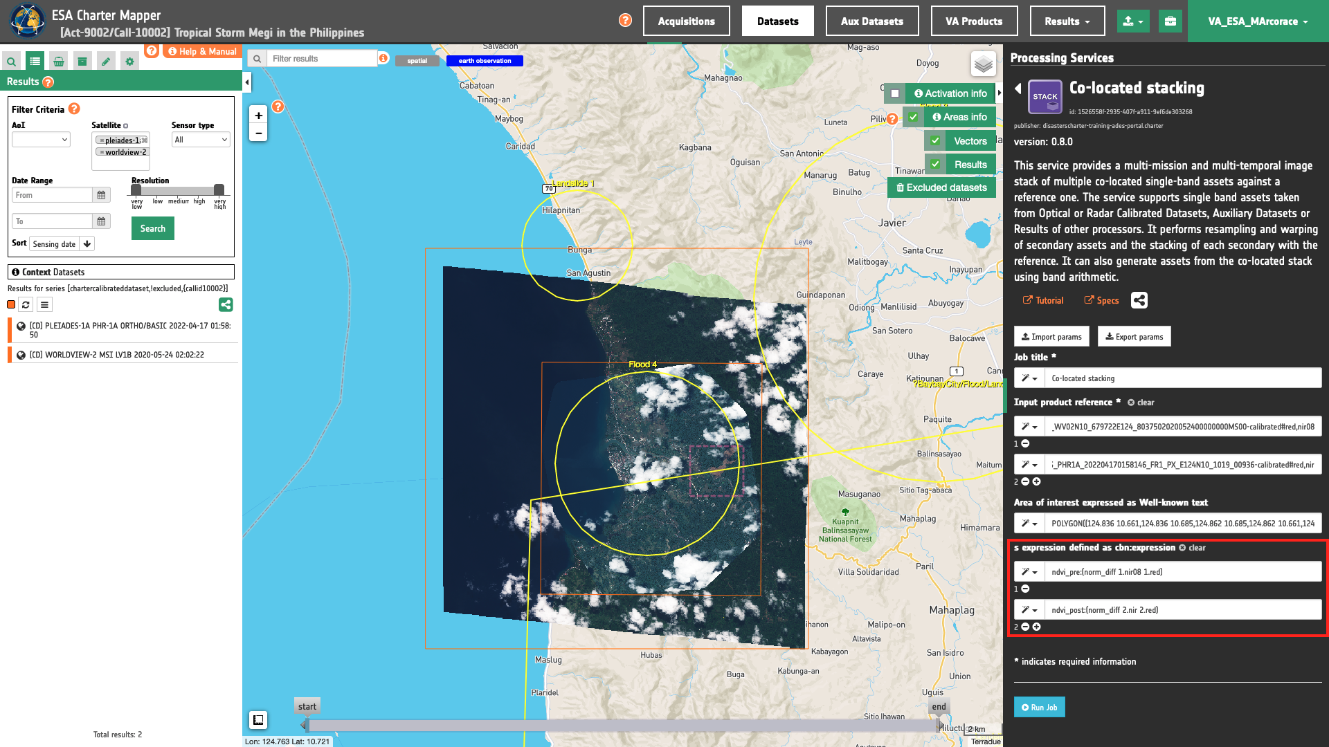
Warning
S-expressions inserted by the user must be given within brackets.
Note
This parameter is optional.
Run the job
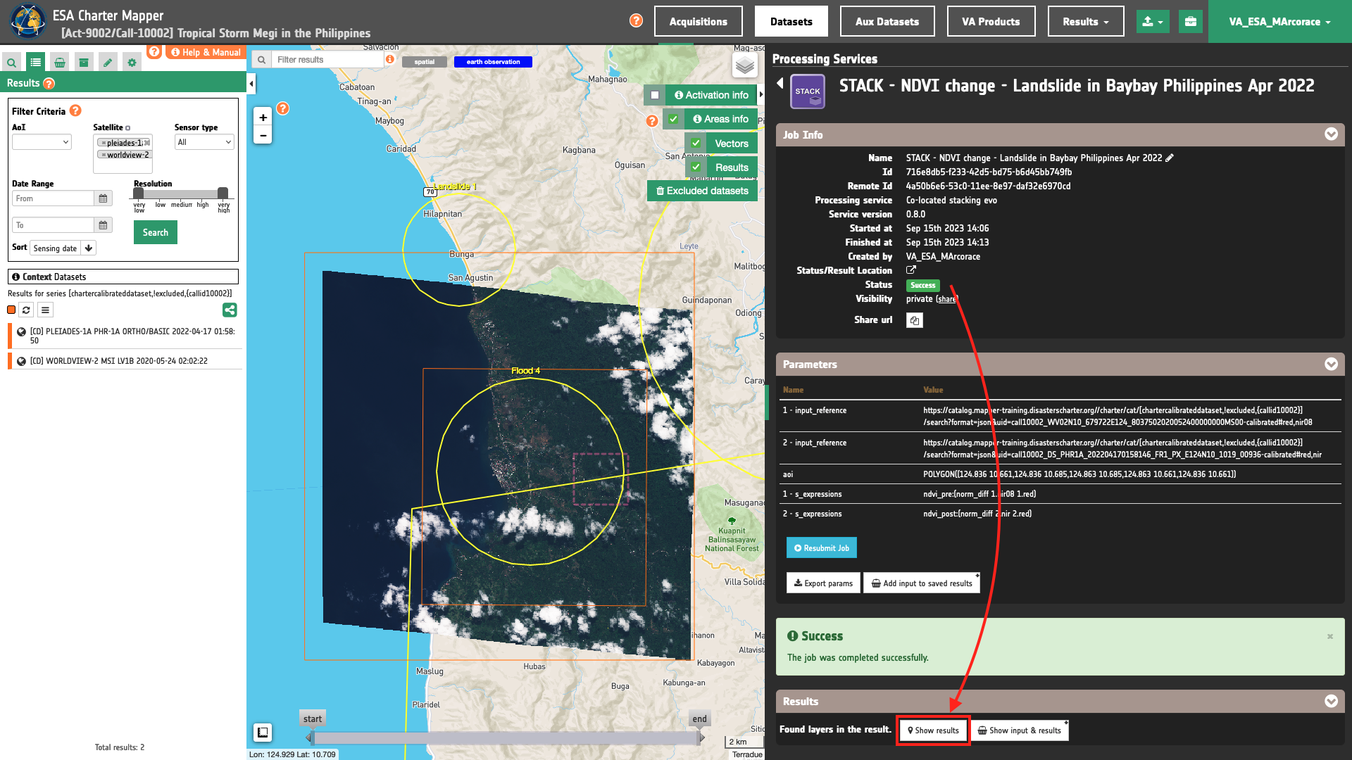
Click on the button Run Job and see the Running Job. You can monitor job progress through the progress bar.

Results: download and visualization
Once the job is completed, click on the button Show results at the bottom of the processing service panel.
Tip
You can also save the parameters employed in this job by clicking on the Export params button in the right panel. This allows you to copy all your entries to the clipboard. This is meant to be used for a quick re-submission of a similar job after a fine tuning of the parameters (e.g. to add a color formula later).
Below is reported the syntax which includes all the parameters employed in this example.
{
   "input_reference": [
      "https://catalog.mapper-training.disasterscharter.org//charter/cat/[chartercalibrateddataset,!excluded,{callid10002}]/search?format=json&uid=call10002_WV02N10_679722E124_8037502020052400000000MS00-calibrated#red,nir08",
      "https://catalog.mapper-training.disasterscharter.org//charter/cat/[chartercalibrateddataset,!excluded,{callid10002}]/search?format=json&uid=call10002_DS_PHR1A_202204170158146_FR1_PX_E124N10_1019_00936-calibrated#red,nir"
   ],
   "aoi": "POLYGON((124.836 10.661,124.836 10.685,124.863 10.685,124.863 10.661,124.836 10.661))",
   "s_expressions": [
      "ndvi_pre:(norm_diff 1.nir08 1.red)",
      "ndvi_post:(norm_diff 2.nir 2.red)"
   ]
}
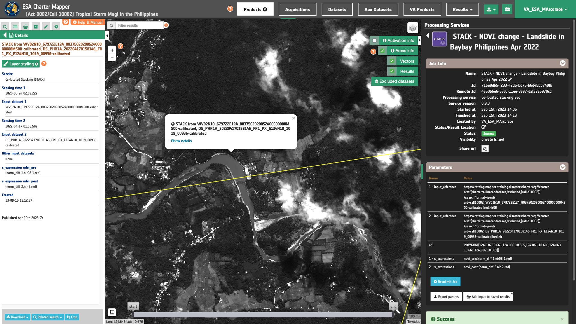
Visualization
See the result on the map. The preview appears within the area defined in the spatial filter.
Warning
STACK does not currently provide a visual product (overview). Thus, the preview in the map is made by default with a RGB composite taking the first 3 single-band assets generated as product by the service.
To get more information about the product just click on the preview in the map, a bubble showing the name of the layer Co-located stack from WV02N10_679722E124_8037502020052400000000MS00-calibrated, DS_PHR1A_202204170158146_FR1_PX_E124N10_1019_00936-calibrated will appear and then click on the Show details button.
Under Select Assets you can select and visualize in the map all the input single band assets 1.red,1.nir08, 2.red, 2.nir and the assets generated with the s-expressions ndvi_pre and ndvi_post.
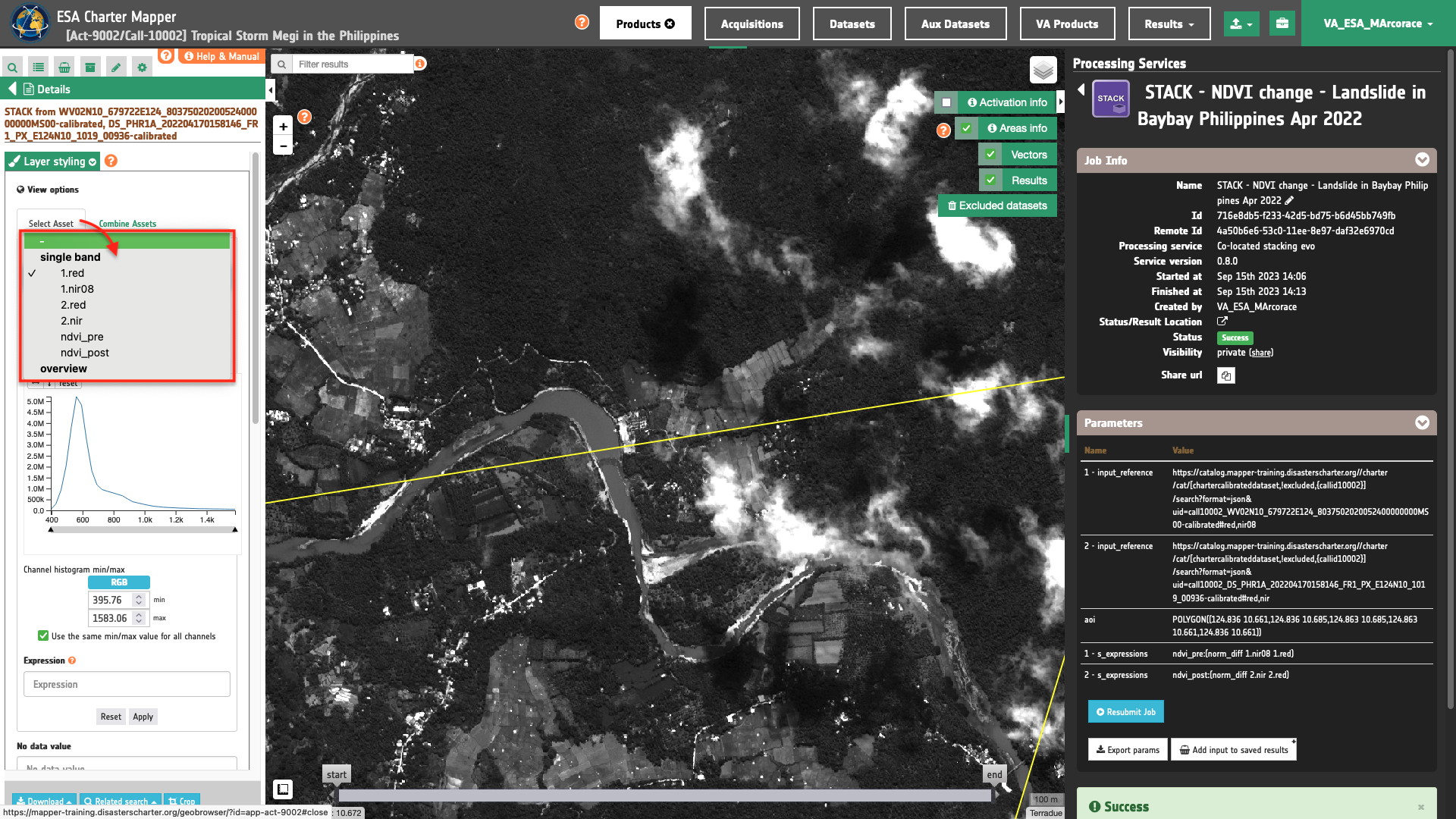
In the left panel under the result Details is possible to customize the overview on the fly by clicking on Layer Styling and Combine Assets. As an example under Combine Assets you can create on the fly a Red-Cyan band composite by setting the ndwi_post band in the red channel, and ndwi_pre in the green and blue channels.
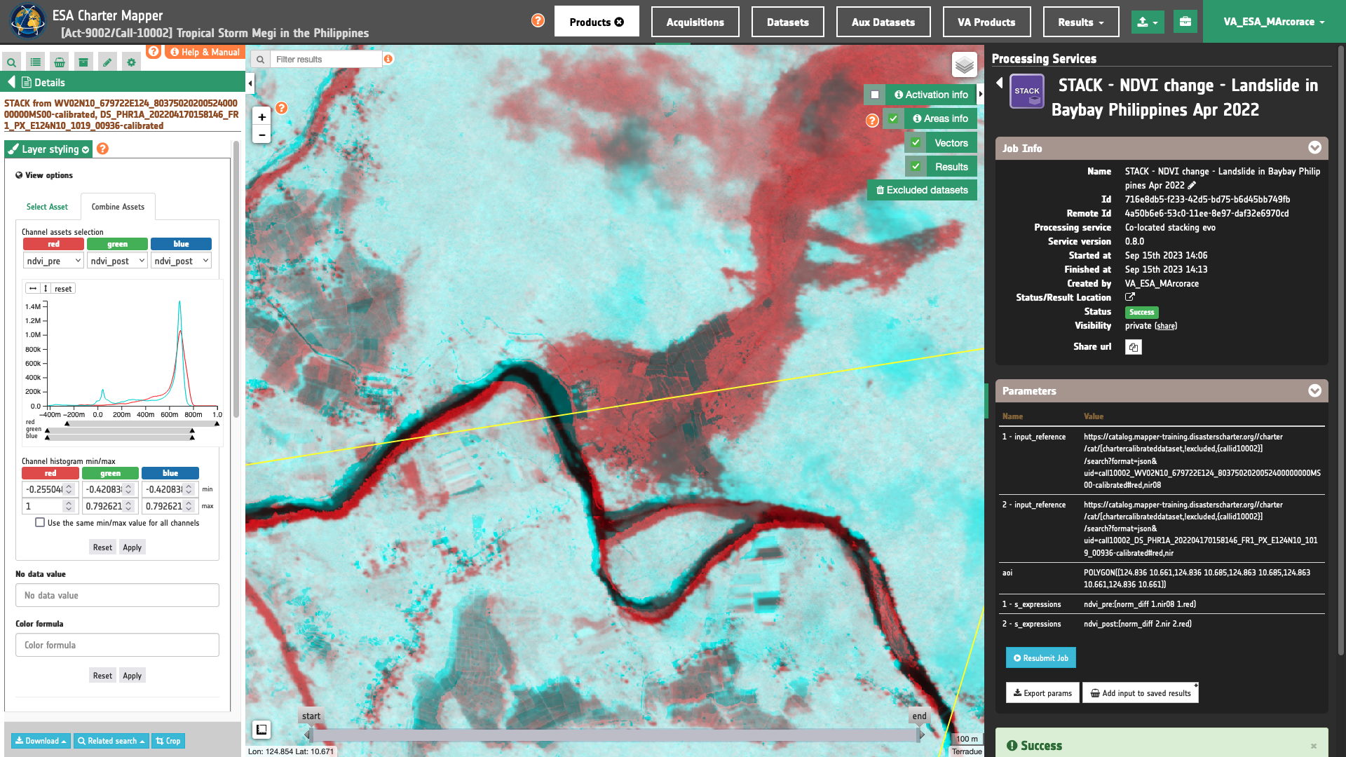
This Red-Cyan band composite highlights NDVI changes derived from Worldview-2 and Pleiades data. In red is shown the vegetation loss due to a landslide near Baybay.
Warning
When combining reflectance single-band assets under Combine assets please consider the valid range associated with the specific asset. As an example consider [-1,1] for a spectral index from a normalized difference, [0,10000] for TOA reflectances, etc. Valid ranges for all single-band assets can be found here. Min and Max values shall be inserted manually in the Channel histogram min/max boxes.
Download
In this first use case the Co-located stacking (STACK) service returned as output the following products:
- 1.red co-located single-band reflectance asset with CBN
redfrom the first input calibrated dataset, - 1.nir co-located single-band reflectance asset with CBN
nir08from the first input calibrated dataset, - 2.red co-located single-band reflectance asset with CBN
redfrom the second input calibrated dataset, - 2.nir co-located single-band reflectance asset with CBN
nirfrom the second input calibrated dataset, - ndvi_pre NDVI single-band reflectance asset derived from co-located
1.redand1.nir08assets using the first inserted s-expression, - ndvi_post NDVI single-band reflectance asset derived from co-located
2.redand2.nirassets using the second inserted s-expression,
All of them are given as single band GeoTIFF in COG format. These products can be downloaded by clicking on the Download button located at the bottom of the Product Details tab in the left panel.
Use case 2: generate a multi-temporal co-located stack of Sigma Nought assets from the same sensor using SAR EO data and derive multiple water masks
Abstract
This second use case explains how to create a stack of co-located Sigma Nought Assets and and derive multiple water masks.
Find the data using multiple filter criteria
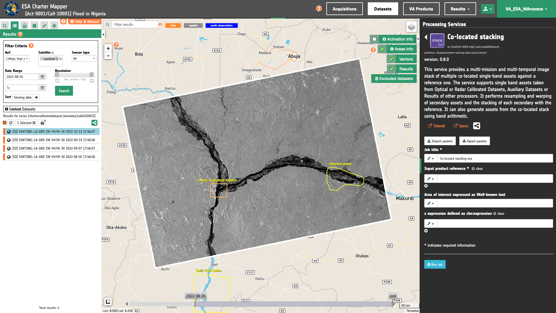
Choose an area in which you want to focus your analysis (e.g in the Kogi state where Niger and Benue rivers meet in Nigeria).
From the Navigation and Search toolbar (located in the upper left side of the map), click on “Spatial Filter” and draw a square around Licungo floodplain, Mozambique. This spatial filter allows you to select only the EO data acquired over this area.
From the top of the left panel, use Filter Criteria to search for Sentinel-1 data collection. Employ also AOI (Lokoja) and time (from 26/08/2022 to 26/08/2022) filters. Once these filters are in place the Result list is updated as shown in the below figure.
Fill the parameters
After the definition of spatial (Lokoja AOI) and time filters (from 26/08/2022 to 26/08/2022), you can apply the co-located stacking, by importing, for example, four single-band assets from four Sentinel-1 Calibrated Datasets. In this example the input calibrated datasets are: Sentinel-1A GRD [CD] acquired on 26/08/2022, 07/09/2022, 19/09/2022, and 13/10/2022.
Job name
Insert as job name:
STACK - S1 Water Masks 26/08-13/10 2022 - Flood in Lokoja, Nigeria
Input single band assets
To derive backscatter average from the below 4 Sentinel-1 calibrated datasets:
-
[CD] SENTINEL-1A GRD IW VV/VH 30 2022-08-26 17:46:06,
-
[CD] SENTINEL-1A GRD IW VV/VH 30 2022-09-07 17:46:07,
-
[CD] SENTINEL-1A GRD IW VV/VH 30 2022-09-19 17:46:06,
-
[CD] SENTINEL-1A GRD IW VV/VH 30 2022-10-13 17:46:07.
it is needed to build a multitemporal STACK using multiple backscatter single band assets (e.g. s0_db_c_vv). To do so, the user shall drag and drop 1 input co-pol backscatter single band asset in VV polarization from each of these 4 Radar Calibrated Datasets.
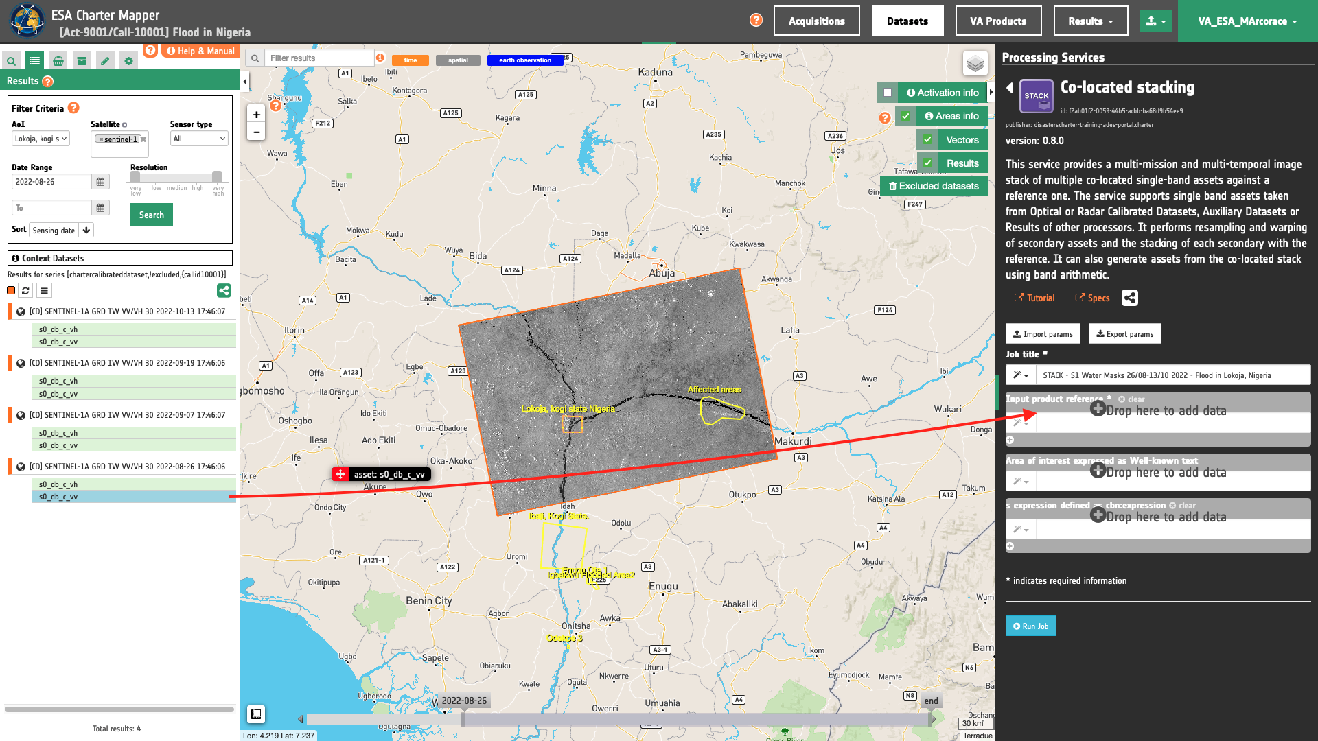
In total dragging and dropping 4 single band assets in the first STACK parameter.
Warning
Drag and drop the single-band asset (e.g. "s0_db_c_vv") and not the Dataset (e.g. "[CD] SENTINEL-1A GRD IW VV/VH 108 2022-02-09 03:00:31") into the Input single band asset(s) field.
Being the 3 input assets originated from 3 different Radar Calibrated Datasets the prefix of each pair of assets will be 1, 2, and 3 according to the order in which they are specified in input.
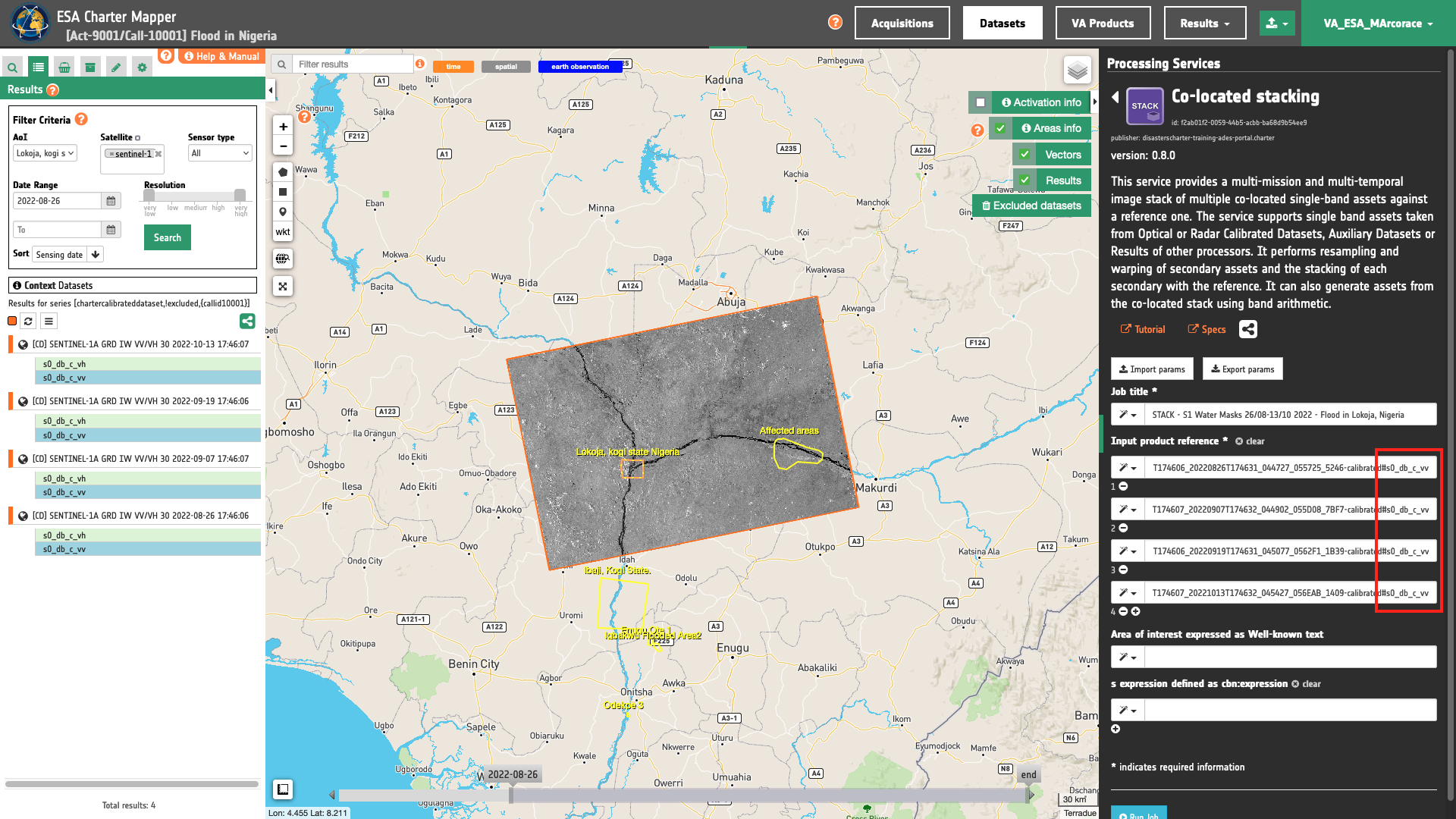
Thus when employing these single band assets in band arithmetic each of them shall be defined as:
-
1.s0_db_c_vv -
2.s0_db_c_vv -
3.s0_db_c_vv -
4.s0_db_c_vv
Tip
Always check the list of CBNs available in a Calibrated Dataset when dragging and dropping the single-band assets. A TerraSAR-X Calibrated Dataset does not have a s0_db_c_vv asset but could have a s0_db_x_hh one.
Note
SAR CBNs for radar backscatter used in the ESA Charter Mapper can be found here.
Area of interest expressed as Well-known text
The “Area of interest as Well Known Text” can be defined by using the drawn polygon defined with the area filter.
Tip
In the definition of “Area of interest as Well Known Text” it is possible to apply as AOI the drawn polygon defined with the area filter. To do so, click on the button in the left side of the "Area of interest expressed as Well-known text" box and select the option AOI from the list. The platform will automatically fill the parameter value with the rectangular bounding box which is taken from the current search area in WKT format.
Note
This parameter is optional.
S-expression
The remaining optional parameter to be filled in is the one dedicated for generating new bands from the ones present in the image stack using s-expressions. In STACK a new band generated from the image stack is defined with a band name and it's associated s-expression separated by a colon : .
output_band_name:(s-expression)
The 4 new Assets to be generated are the water mask derived from the binarization of each input sigma nought asset. To compute them provide the following 4 s-expressions that are using the four input assets (Sigma Nought co-pol of each acquisition).
For instance the s-expression:
water_mask_20220826:(where (<= 1.s0_db_c_vv -16) 1 0)
can be used to make the binarization of radar backscatter for the first single band asset.
In this s-expression the where operator is then applied to derive a binary mask satisfying this condition: Sigma0 <= signed threshold in db. The value -23 represents the threshold for Sigma Nought in dB.
The input is the 1.s0_db_c_vv single band asset representing Sigma Nought in dB from systematic Radar Calibration of a C-band intensity image in VV polarization. The output water_mask_20220826 is a single band binary mask derived from this input backscatter asset with the provided s-expression.
Insert the following 4 s-expressions to derive a water mask from each single band asset.
water_mask_20220826:(where (<= 1.s0_db_c_vv -16) 1 0)
water_mask_20220907:(where (<= 2.s0_db_c_vv -16) 1 0)
water_mask_20220919:(where (<= 3.s0_db_c_vv -16) 1 0)
water_mask_20221013:(where (<= 4.s0_db_c_vv -16) 1 0)
Warning
S-expressions inserted by the user must be given within brackets.
Note
This parameter is optional.
Run the job
Click on the button Run Job and see the Running Job. You can monitor job progress through the progress bar.
Results: download and visualization
Once the job is completed, click on the button Show results at the bottom of the processing service panel.
Below is reported the syntax which includes all the parameters employed in this example.
{
   "input_reference": [
      "https://catalog.mapper-training.disasterscharter.org//charter/cat/[chartercalibrateddataset,!excluded,{callid10001}]/search?format=json&uid=call10001_S1A_IW_GRDH_1SDV_20220826T174606_20220826T174631_044727_055725_5246-calibrated#s0_db_c_vv",
      "https://catalog.mapper-training.disasterscharter.org//charter/cat/[chartercalibrateddataset,!excluded,{callid10001}]/search?format=json&uid=call10001_S1A_IW_GRDH_1SDV_20220907T174607_20220907T174632_044902_055D08_7BF7-calibrated#s0_db_c_vv",
      "https://catalog.mapper-training.disasterscharter.org//charter/cat/[chartercalibrateddataset,!excluded,{callid10001}]/search?format=json&uid=call10001_S1A_IW_GRDH_1SDV_20220919T174606_20220919T174631_045077_0562F1_1B39-calibrated#s0_db_c_vv",
      "https://catalog.mapper-training.disasterscharter.org//charter/cat/[chartercalibrateddataset,!excluded,{callid10001}]/search?format=json&uid=call10001_S1A_IW_GRDH_1SDV_20221013T174607_20221013T174632_045427_056EAB_1409-calibrated#s0_db_c_vv"
   ],
   "aoi": "POLYGON((6.13 7.499,6.13 8.614,8.163 8.614,8.163 7.499,6.13 7.499))",
   "s_expressions": [
      "water_mask_20220826:(where (<= 1.s0_db_c_vv -16) 1 0)",
      "water_mask_20220907:(where (<= 2.s0_db_c_vv -16) 1 0)",
      "water_mask_20220919:(where (<= 3.s0_db_c_vv -16) 1 0)",
      "water_mask_20221013:(where (<= 4.s0_db_c_vv -16) 1 0)"
   ]
}
Visualization
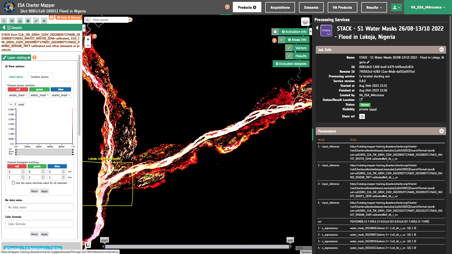
See the result on the map. The preview appears within the area defined in the spatial filter.
Warning
STACK does not currently provide a visual product (overview). Thus, the preview in the map is made by default with a RGB composite taking the first three single-band assets generated as product by the service.
To get more information about the product just click on the preview in the map, a bubble showing the name of the layer STACK from S1A_IW_GRDH_1SDV_20220826T174606_20220826T174631_044727_055725_5246-calibrated, S1A_IW_GRDH_1SDV_20220907T174607_20220907T174632_044902_055D08_7BF7-calibrated and other datasets or products will appear and then click on the Show details button.
In the left Result panel under Details is possible to customize the overview on the fly by clicking on Layer Styling and Combine Assets. As an example under Combine Assets you can create on the fly RGB band composite by setting water_mask_20221013 in the red channel, water_mask_20220919 in the green channel, and water_mask_20220907 in the blue channel.
Warning
When combining backscatter single-band assets under Combine assets please consider the valid range associated with the specific asset. As an example consider [-20,0] for a co-pol backscatter in C-band. Valid ranges for all single-band assets can be found here. Min and Max values shall be inserted manually in the Channel histogram min/max boxes.
Download
In this second use case the Co-located stacking (STACK) service returned as output the following products:
- 1.s0_db_c_vv co-located single-band Sigma Nought asset with CBN
s0_db_c_vvfrom the 1st input calibrated dataset, - 2.s0_db_c_vv co-located single-band Sigma Nought asset with CBN
s0_db_c_vvfrom the 2nd input calibrated dataset, - 3.s0_db_c_vv co-located single-band Sigma Nought asset with CBN
s0_db_c_vvfrom the 3rd input calibrated dataset, - 4.s0_db_c_vv co-located single-band Sigma Nought asset with CBN
s0_db_c_vvfrom the 4th input calibrated dataset, - water_mask_20220826 single-band asset derived from the binarization of the
1.s0_db_c_vvasset using the 1st inserted s-expression, - water_mask_20220907 single-band asset derived from the binarization of the
2.s0_db_c_vvasset using the 1st inserted s-expression, - water_mask_20220919 single-band asset derived from the binarization of the
3.s0_db_c_vvasset using the 1st inserted s-expression, - water_mask_20221013 single-band asset derived from the binarization of the
4.s0_db_c_vvasset using the 1st inserted s-expression,
All of them are given as single band GeoTIFF in COG format. These products can be downloaded by clicking on the Download button located at the bottom of the Product Details tab in the left panel.
Use case 3: generate coherence loss map from a co-located stack of pre- and post-event coherence assets derived from the same sensor
Abstract
This third use case explains how to create a co-located stack of two interferometric coherence assets, derive the difference from them and use it for binarization to estimate the coherence loss.
Find and access a Result from other on-demand services
Select the area for which you want to do an analysis e.g. over the Southern part of Turkey near the border with Syria. In this use case two Results from the SAR-COIN are used to assess the change in coherence that occurred after the 7.8-magnitude earthquake of 06/02/2023.
Access two successful SAR-COIN jobs in the Right Panel Processing Services under the Jobs tab. Alternatively, the same SAR-COIN processing results can also be listed in the left panel by clicking on My results or Shared results under the Results data context.
Note
A description of the Results data context button can be found here.
Select a pair of SAR-COIN Results to be used for the Co-located Stacking.
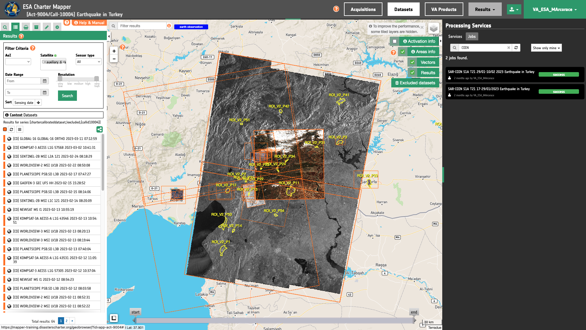
In this example the selected two SAR-COIN results derived from two pairs of Sentinel-1 SLC Datasets are:
-
Reference SAR-COIN Result (before earthquake):
COIN S1A T14 17-29/01/2023 Turkey Earthquake -
Secondary SAR-COIN Result (after earthquake):
COIN S1A T14 29/01-10/02 2023 Turkey Earthquake
The first SAR-COIN Result is derived from the following SLC products (acquired both before the earthquake):
-
Reference:
S1A_IW_SLC__1SDV_20230117T033426_20230117T033454_046818_059D16_1A0C -
Secondary:
S1A_IW_SLC__1SDV_20230129T033427_20230129T033455_046993_05A2FE_6FF2
The second SAR-COIN Result instead is derived from the following SLC interferometric pair (reference as the secondary of the first SAR-COIN result and secondary after the event):
-
Reference:
S1A_IW_SLC__1SDV_20230129T033427_20230129T033455_046993_05A2FE_6FF2 -
Secondary:
S1A_IW_SLC__1SDV_20230210T033426_20230210T033454_047168_05A8CD_FAA6
Open the first SAR-COIN job and from the Job details click on Show results. A feature will appear under the Results list.
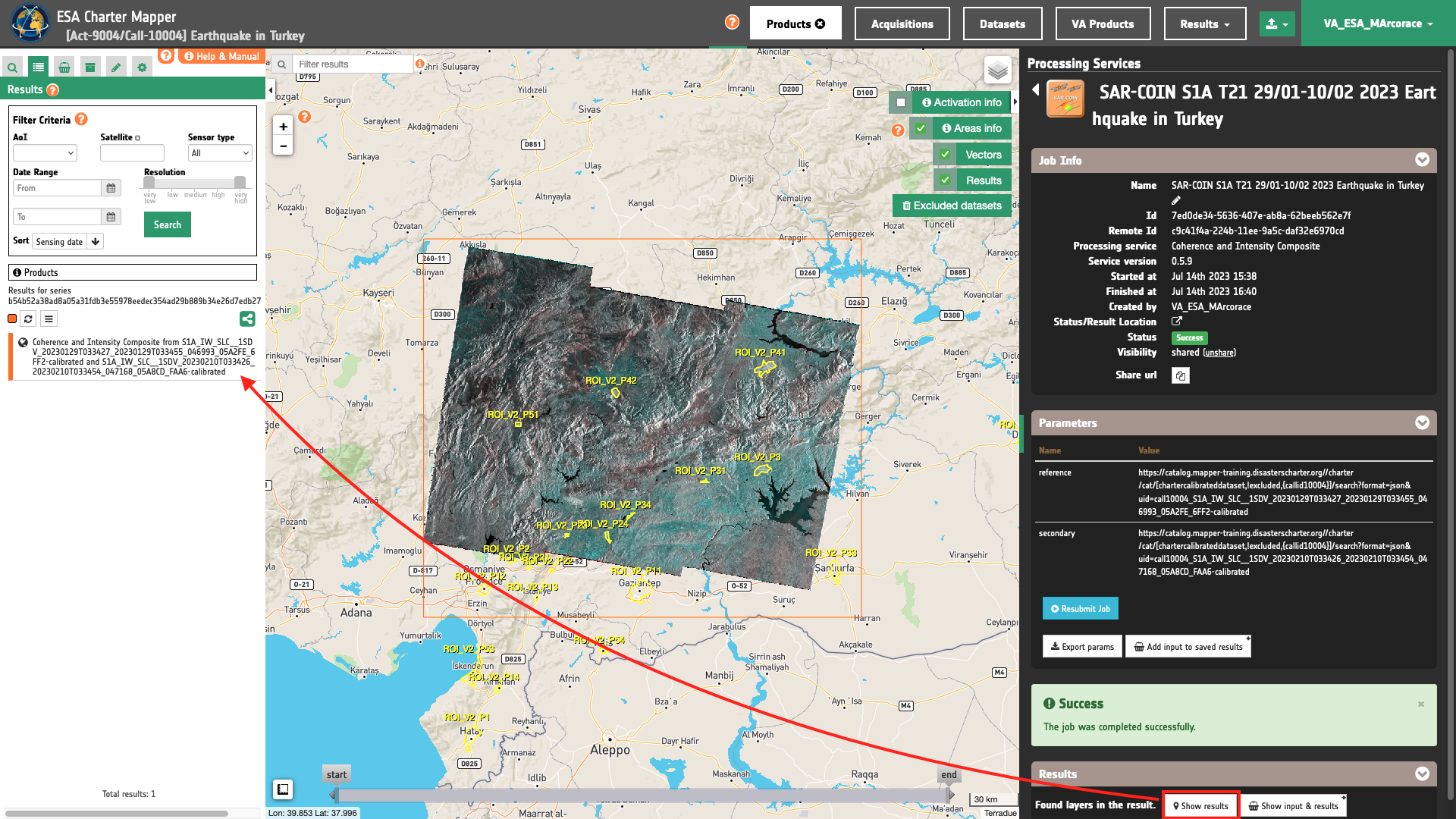
Drag ang drop it into the features basket.
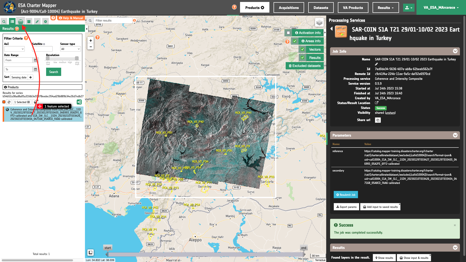
Repeat the same for the second SAR-COIN job. After that the features basket will include the two SAR-COIN results as shown in the below figure.
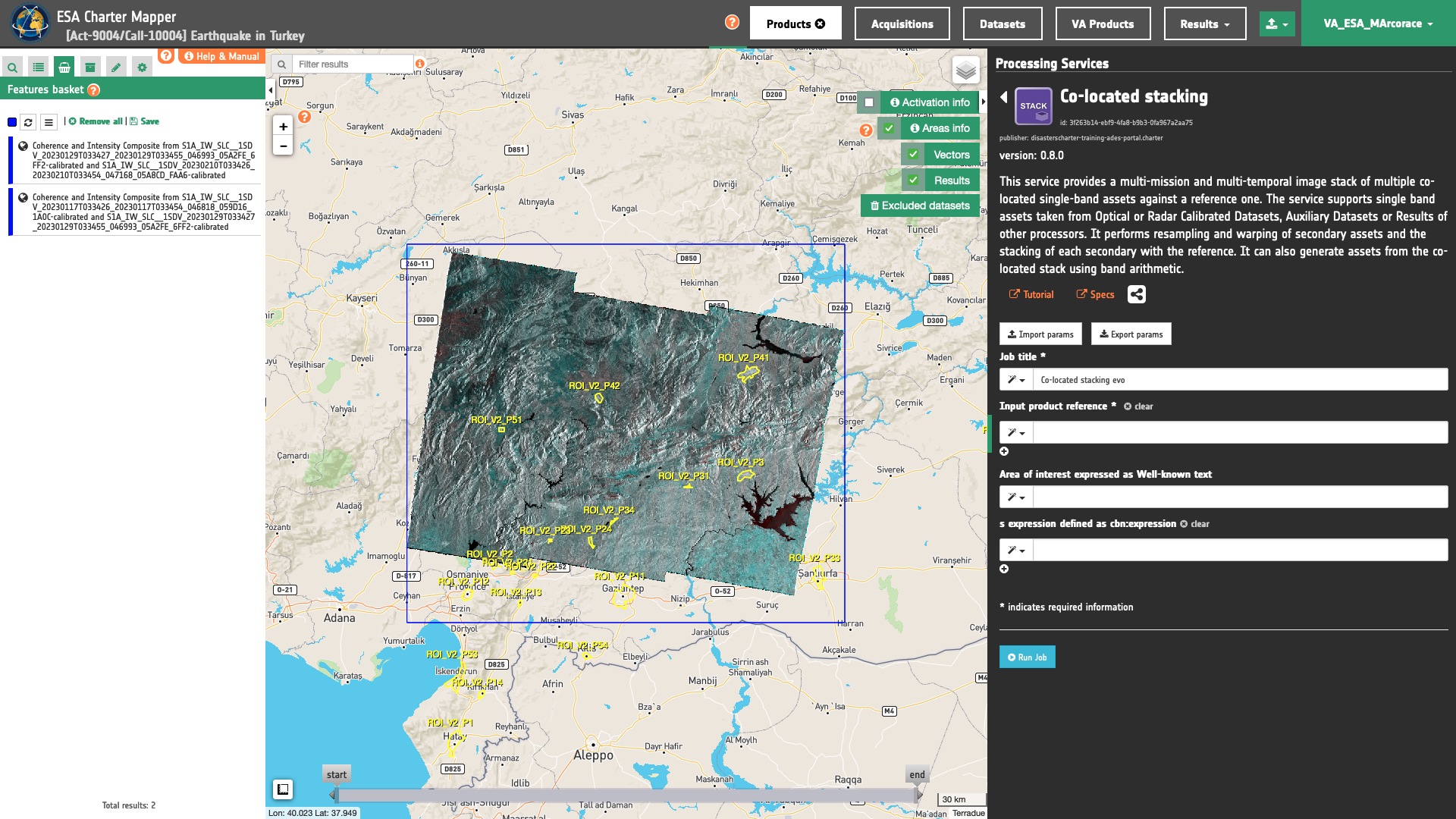
Job name
Insert as job name:
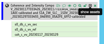
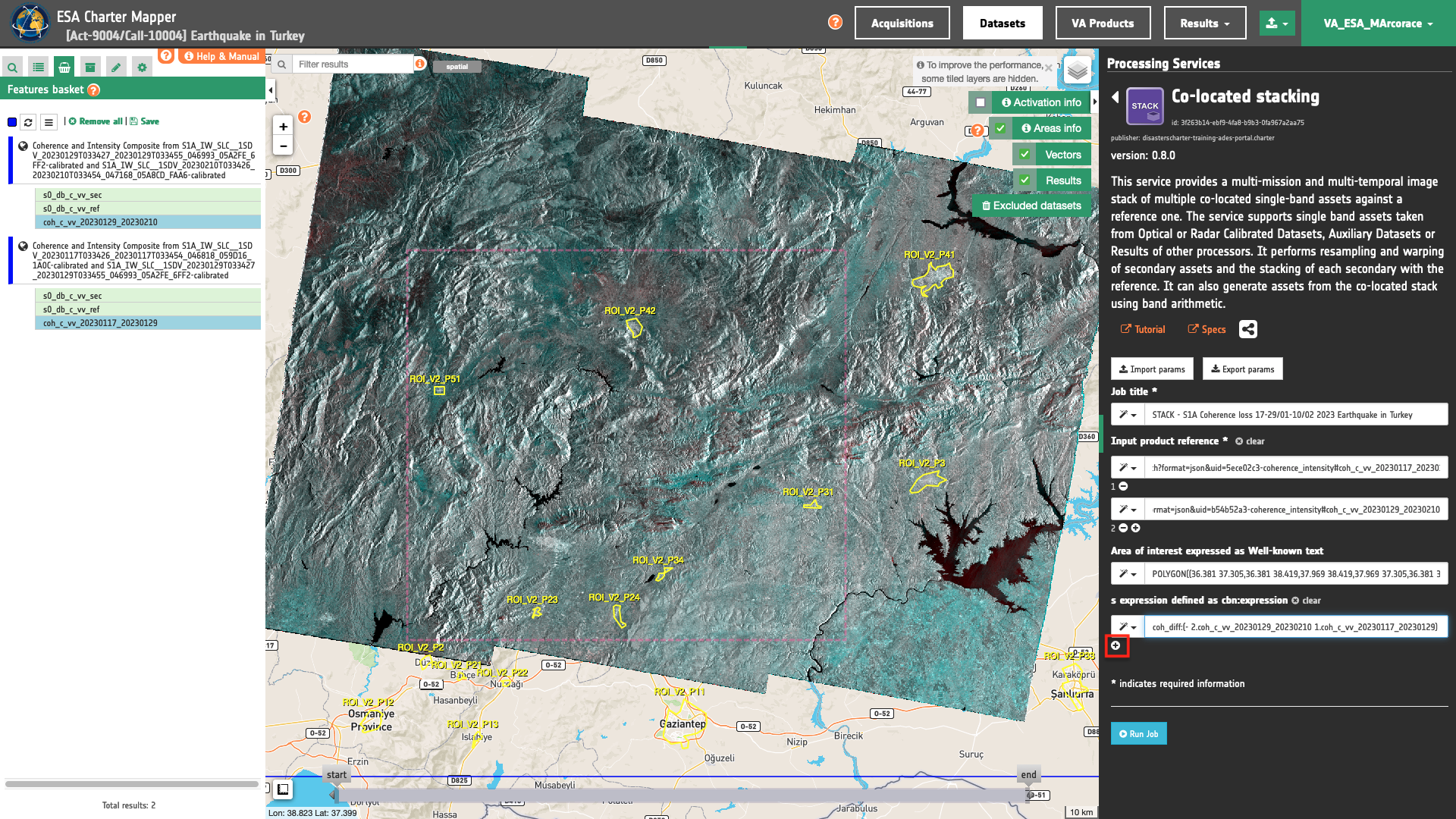
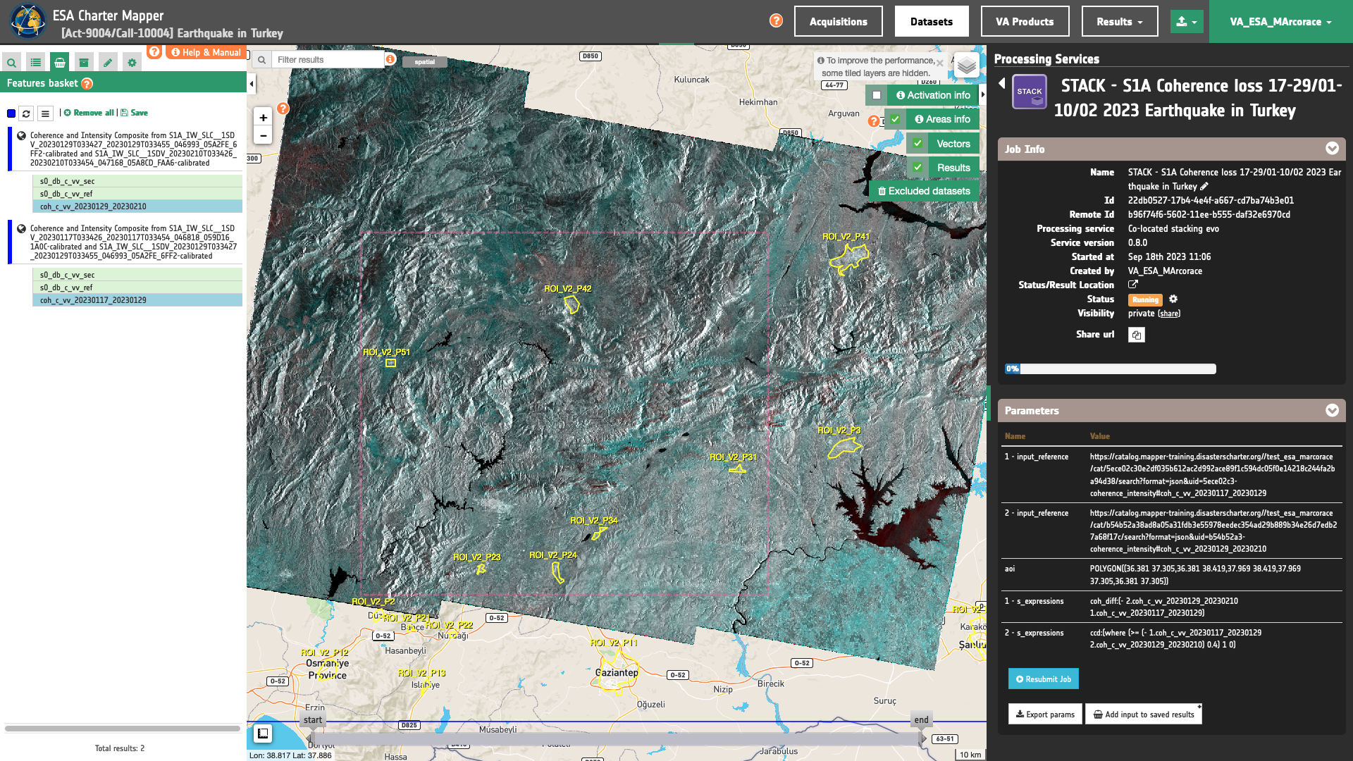
STACK - S1A Coherence loss 17-29/01-10/02 2023 Earthquake in Turkey
Input single band assets
To build a multitemporal STACK using a pair of coherence assets (coh_B_PP_YYYYMMDD_YYYYMMDD) and coherence loss mask from the below 2 SAR-COIN Results:
-
COIN S1A T14 17-29/01/2023 Turkey Earthquake, -
COIN S1A T14 29/01-10/02 2023 Turkey Earthquake.
the user shall drag and drop 1 input coherence single band asset from each of these 2 Results in the "Input single band asset(s)” field.
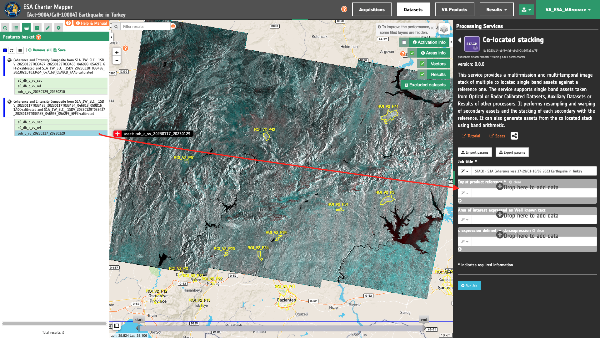
In total dragging and dropping 2 assets in the first STACK parameter.
Warning
Drag and drop the single band asset (e.g. coh_c_vv_20230117_20230129) and not the Result (e.g. Coherence and Intensity Composite from S1A_IW_SLC__1SDV_20230117T033426_20230117T033454_046818_059D16_1A0C-calibrated and S1A_IW_SLC__1SDV_20230129T033427_20230129T033455_046993_05A2FE_6FF2-calibrated) into the Input single band asset(s) field.
Being the 2 input assets originated from 2 different OPT-Index Results the prefix of each asset will be 1, and 2 according to the order in which they are specified in input. Thus when employing these single band assets in band arithmetic each of them shall be defined as:
-
1.coh_c_vv_20230117_20230129 -
2.coh_c_vv_20230129_20230210

Warning
Drag and drop the single-band asset (e.g. "ndvi") and not the Result (e.g. "OPT-Index - S2 13/07/2021 Dixie Fire, US") into the Input single band asset(s) field.
Tip
Always check the name of assets available in a Result of a processing-service (e.g. SAR-COIN) before defining the list of single-band assets. A Result from SAR-COIN includes multiple single-band assets with different names.
S-expression
The remaining optional parameter to be filled in is the one dedicated for generating new bands from the ones present in the image stack using s-expressions. In STACK a new band generated from the image stack is defined with a band name and it's associated s-expression separated by a colon : .
output_band_name:(s-expression)
The 2 new Assets to be generated are the coherence difference and the binary mask representing coherence loss derived from thresholding of coherence difference.
To compute them provide the following 2 s-expressions that are using the two input assets (coherence from each interferometric SLC pair). For instance coh_diff is the arithmetic difference of the two coherence assets (coherence2 - coherence1) and ccd as coherent change detection is a binarization of coherence difference (where (coh_diff >= threshold) set 1 else 0).
coh_diff:(- 2.coh_c_vv_20230129_20230210 1.coh_c_vv_20230117_20230129)
ccd:(where (>= (- 1.coh_c_vv_20230117_20230129 2.coh_c_vv_20230129_20230210) 0.4) 1 0)
Hint
After the insertion of the first s-expression, click on the below + icon to insert a second s-expression.
Note
The threshold of 0.4 in the 2nd s-expression is just an example. It means considering all pixels of AOI having difference in coherence minor than -0.4. If needed, modify it as appropriate.
Run the job
Click on the button Run Job and see the Running Job.
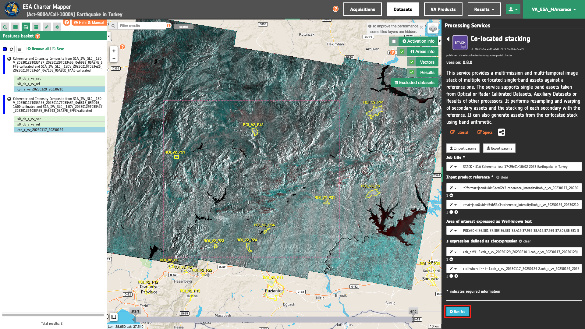
You can monitor job progress through the progress bar.
Results: download and visualization
Once the job is completed, click on the button Show results at the bottom of the processing service panel.
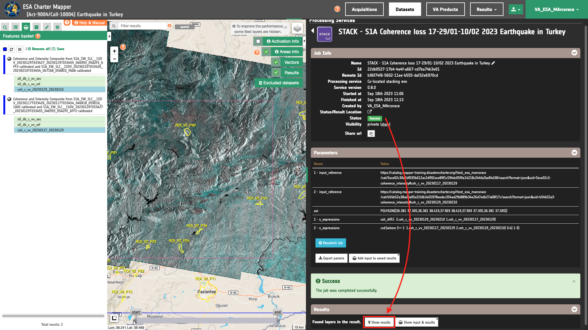
Below is reported the syntax which includes all the parameters employed in this example.
{
   "input_reference": [
      "https://catalog.mapper-training.disasterscharter.org//test_esa_marcorace/cat/5ece02c30e2df035b612ac2d992ace89f1c594dc05f0e14218c244fa2ba94d38/search?format=json&uid=5ece02c3-coherence_intensity#coh_c_vv_20230117_20230129",
      "https://catalog.mapper-training.disasterscharter.org//test_esa_marcorace/cat/b54b52a38ad8a05a31fdb3e55978eedec354ad29b889b34e26d7edb27a68f17c/search?format=json&uid=b54b52a3-coherence_intensity#coh_c_vv_20230129_20230210"
   ],
   "aoi": "POLYGON((36.381 37.305,36.381 38.419,37.969 38.419,37.969 37.305,36.381 37.305))",
   "s_expressions": [
      "coh_diff:(- 2.coh_c_vv_20230129_20230210 1.coh_c_vv_20230117_20230129)",
      "ccd:(where (>= (- 1.coh_c_vv_20230117_20230129 2.coh_c_vv_20230129_20230210) 0.4) 1 0)"
   ]
}
Visualization
See the result on the map. The preview appears within the area defined in the spatial filter.
Warning
STACK does not currently provide a visual product (overview). Thus, the preview in the map is made by default with a RGB composite taking the first three single-band assets generated as product by the service.
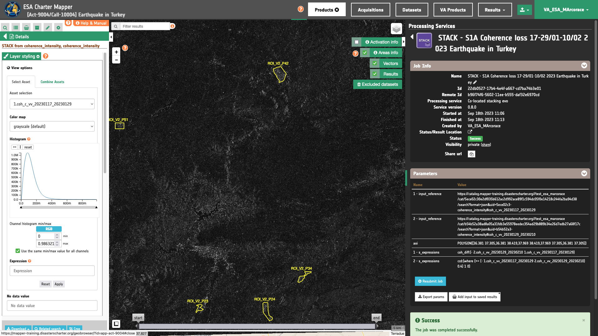
To get more information about the product just click on the preview in the map, a bubble showing the name of the layer Co-located stack from coherence_intensity, coherence_intensity will appear and then click on the Show details button. Under Select Assets you can select and visualize in the map all the input single band assets 1.coh_c_vv_20230117_20230129,2.coh_c_vv_20230129_20230210 and the assets generated with the s-expressions coh_diff and ccd.
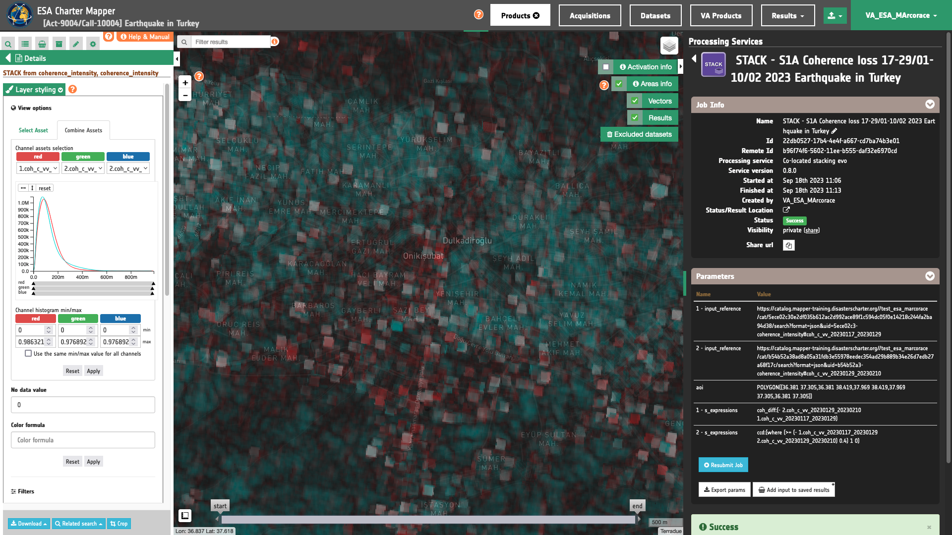
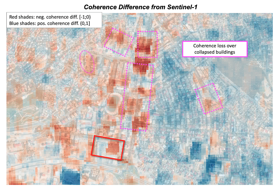
Red-Cyan coherence composite
In the left Result panel under Details is possible to create an overview on the fly from co-located assets by clicking on Layer Styling and Combine Assets. As an example under Combine Assets you can create on the fly Red-Cyan coherence band composite by setting 1.coh_c_vv_20230117_20230129 in the red channel, and 2.coh_c_vv_20230129_20230210 in the green and blue channels.
Coherence difference single band asset
The difference in coherence generated from the two co-located coh_c_vv_20230117_20230129 and coh_c_vv_20230129_20230210 assets with the first s-expression, can be seen in the map by clicking on Layer Styling and under Select Assets by selecting the coh_diff single band asset.
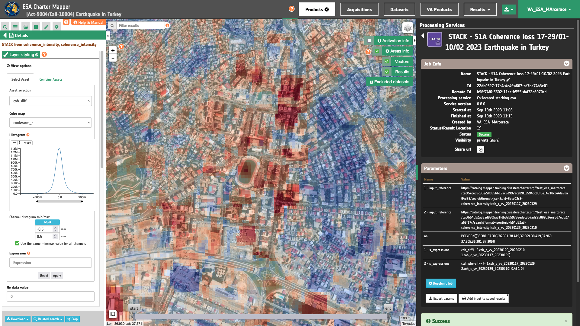
The coh_diff single band asset generated with STACK is displayed in the map using the Select Assets function and the coolwarm_r color map (negative coherence differences in shades of red and positive differences in shades of blue). Min and Max are set to -0.5 and 0.5 respectively.
Coherence loss binary mask single band asset
The result from the binarization of negative coherence difference values (coh_dif < -0.4) obtained with the second s-expression, can be seen in the map by clicking on Layer Styling and under Select Assets by selecting the ccd single band asset.
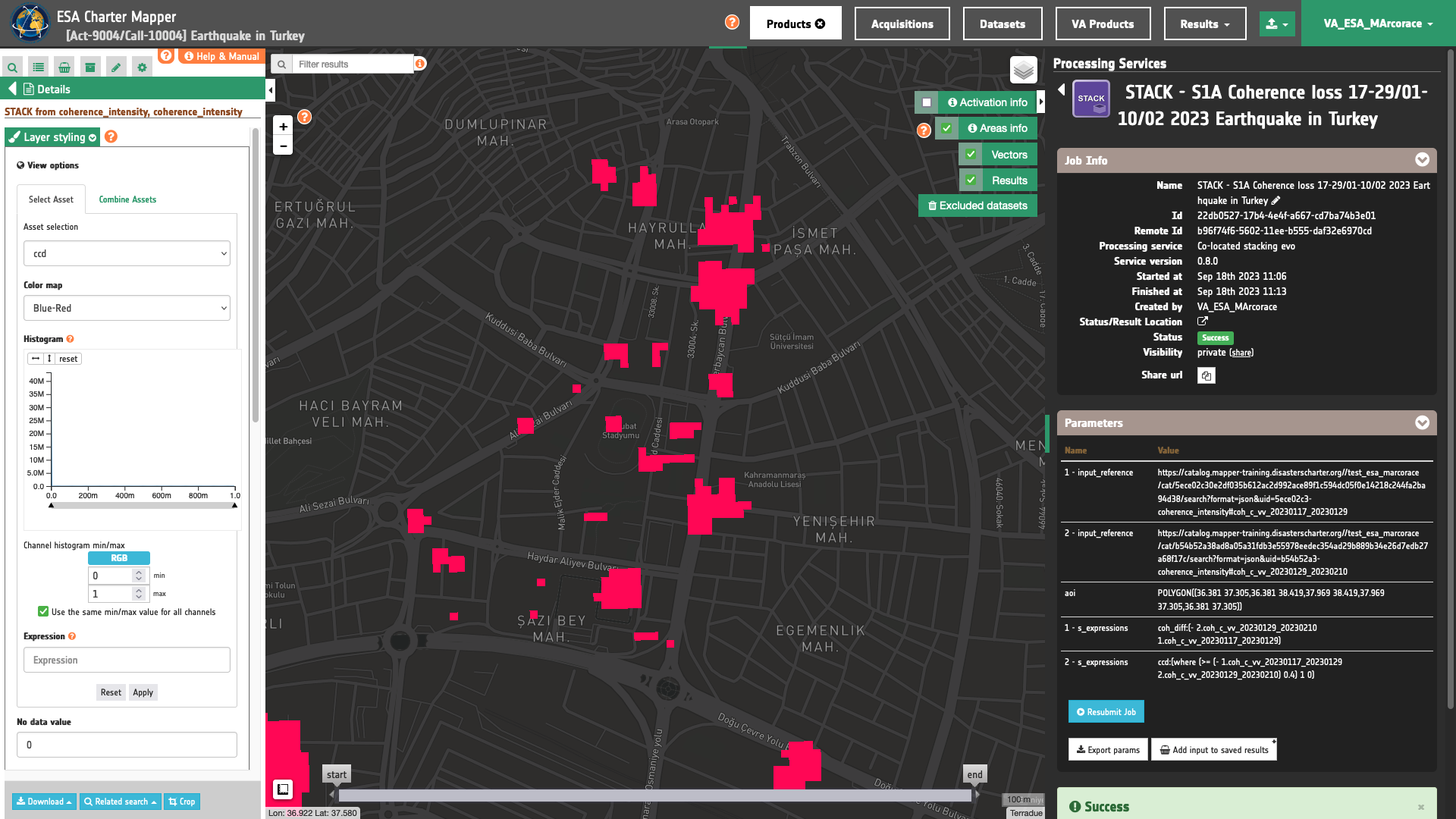
This ccd single band asset generated with STACK is displayed in the map using the Select Assets function, the Blue-Red color map (true values in red), No Data Value set as 0, and brightness filter set as 300%.
Analysis
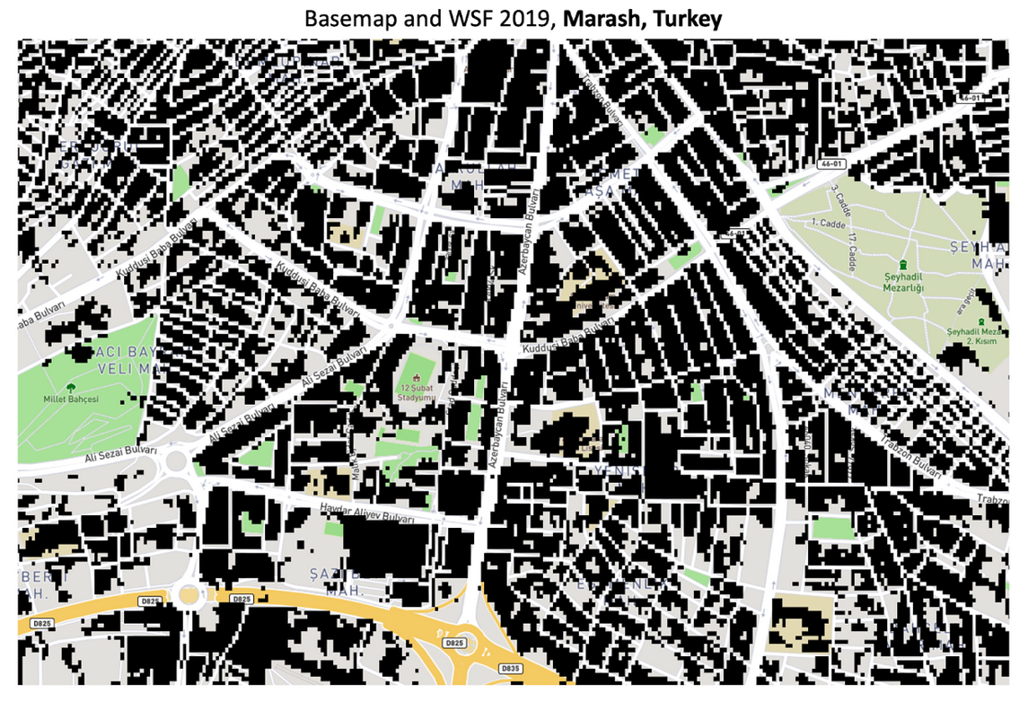
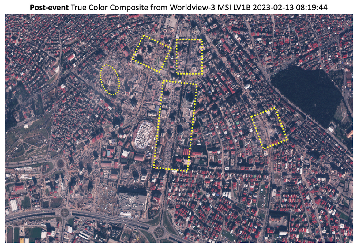
Zoom to the Marash city centre, and superimpose the DLR WSF 2019 global base layer to easily recognize building footprints.
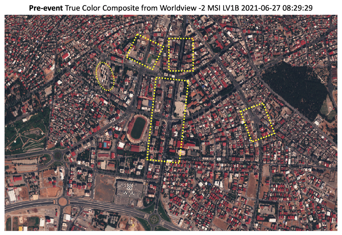
Visually inspect True Colour composites from WorldView-2 and Worldview-3 data acquired before and after the earthquake. In the below images some of the damaged built-up are highlighted in yellow.
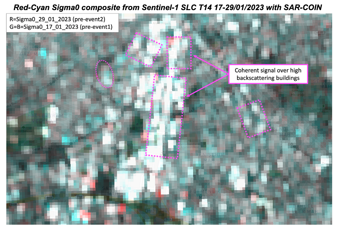
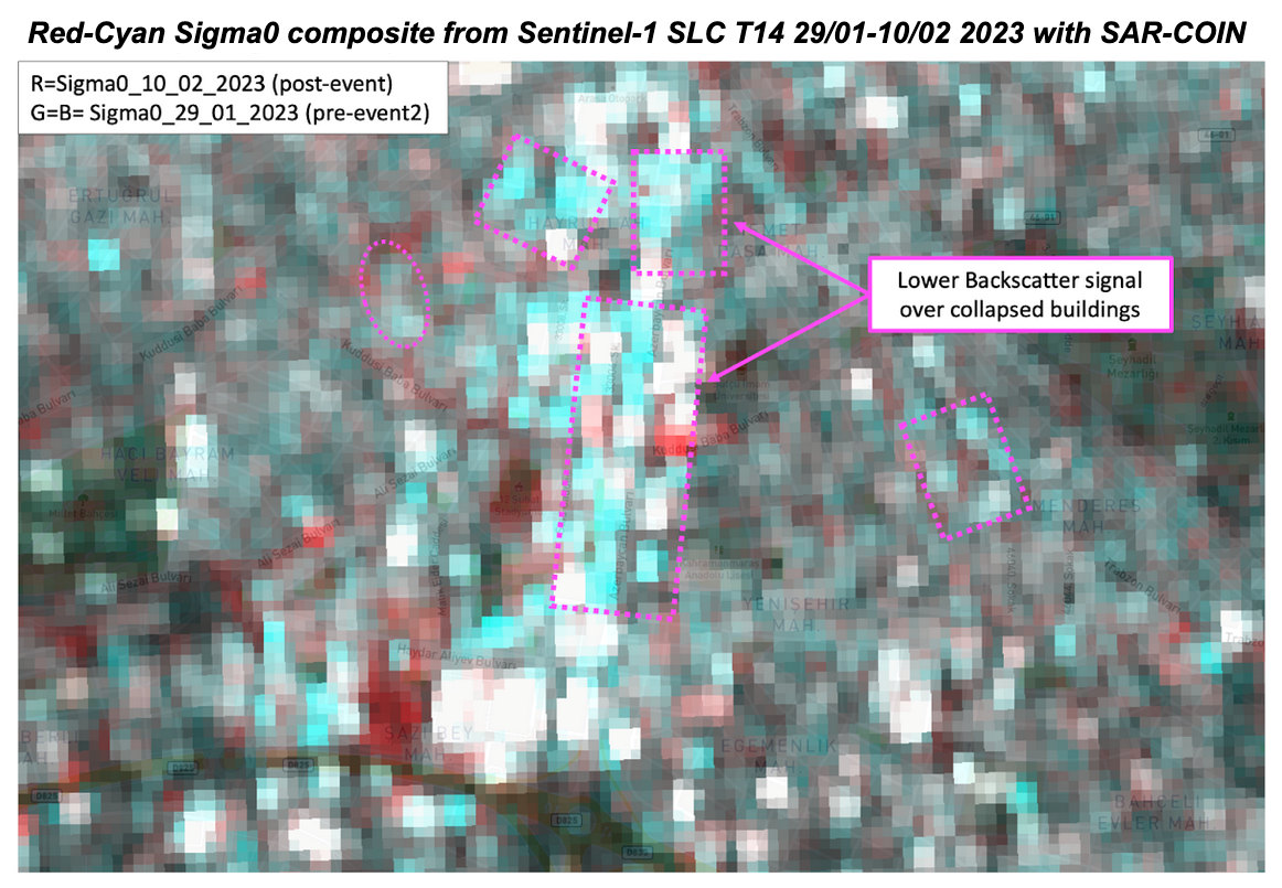
To evaluate backscatter changes before and after the earthquake, from the two SAR-COIN results create on the fly Red-Cyan backscatter band composite by setting the single band asset 1.s0_db_c_vv_sec in the Red channel, and the 2.s0_db_c_vv_ref one in the Green and Blue channels. Apply an image stretch using the following min/max values:
-
Min = -20 dB
-
Max = 5dB
Repeat the same also using the Sigma0 assets from the second SAR-COIN result.
When comparing the top figure with the bottom one a decrease of backscatter (cyan) is shown over collapsed buildings and an increase over debris (red).
When comparing the top figure with the bottom one a decrease of backscatter (cyan) is shown over collapsed buildings and an increase over debris (red).
A quantification of the change in intensity can be further completed outside the ESA Charter Mapper with the Intensity Correlation Difference (ICD) index. Read more about this work in the INGV web news available at www.ingv.it.
The below figure shows a result obtained by the INGV over the same area using acquisitions before and after the earthquake from an higher res SAR sensor, COSMO-SkyMED (Image credit: INGV, ASI).
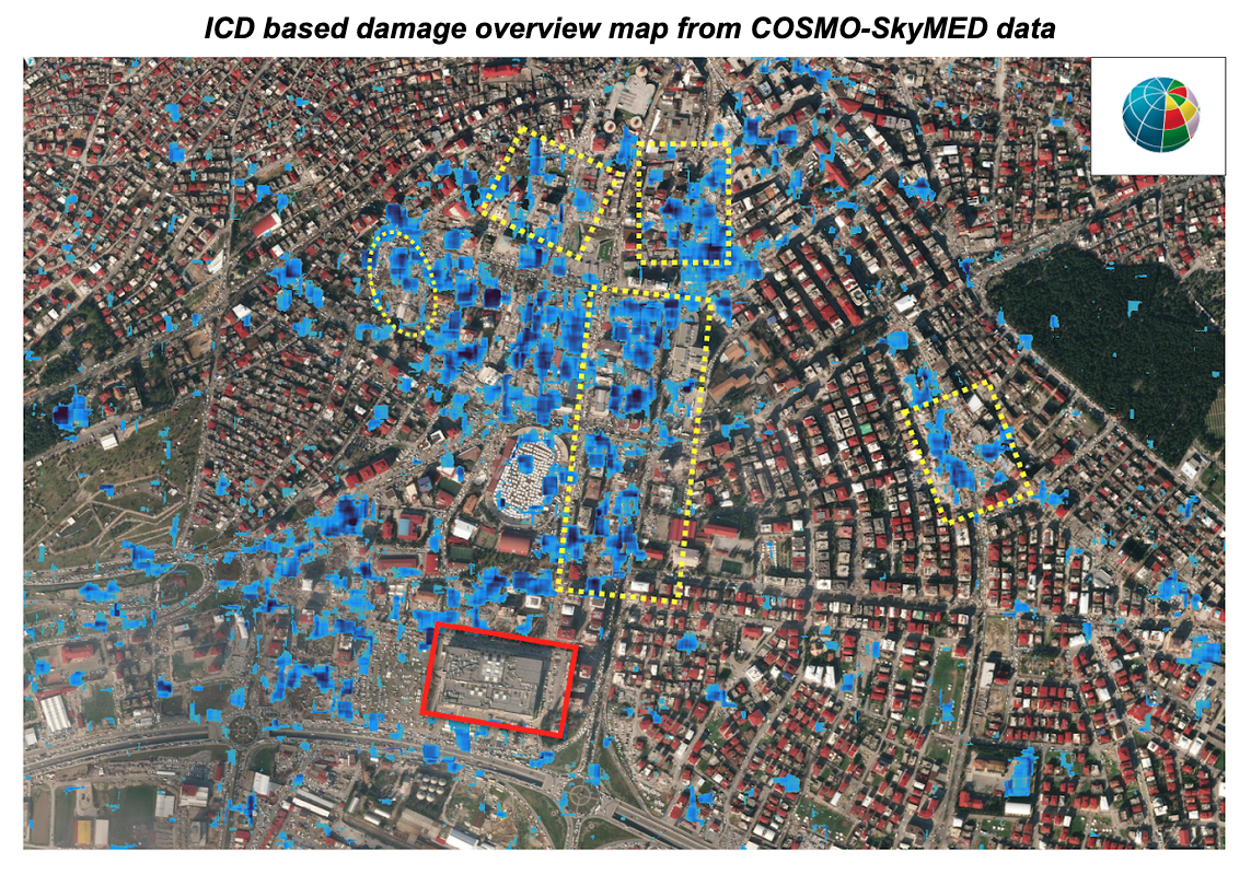
The loss of coherence obtained with the STACK service can further complement the ICD analysis. In fact, the coherence difference analysis also highlights damaged buildings which did not collapse completely, but only partially, e.g. the red rectangle at the bottom of the above figure, that not even the intensity analysis with CSK image was able to detect.
Download
In this fifth use case the Co-located stacking (STACK) service returned as output the following products:
- coh_c_vv_20230117_20230129: single band asset for the co-located
coh_c_vv_20230117_20230129asset from the 1st input Result, - coh_c_vv_20230129_20230210: single band asset for the co-located
coh_c_vv_20230129_20230210coherence asset from the 2nd input Result, - coh_diff single-band asset representing the difference of co-located
coh_c_vv_20230117_20230129andcoh_c_vv_20230129_20230210assets derived with the 1st inserted s-expression, - ccd single-band asset a binary mask ok coherence loss from the difference of co-located
coh_c_vv_20230117_20230129andcoh_c_vv_20230129_20230210assets derived with the 2nd inserted s-expression.
All of them are given as single band GeoTIFF in COG format. These products can be downloaded by clicking on the Download button located at the bottom of the Product Details tab in the left panel.