DISMapper service specifications

Warning

The DISMapper service is still under development but will soon be available in operations.

Service Description

DISaster Mapper (DISMapper) service targets the detection and mapping of sudden/abrupt changes in a landscape triggered by natural disasters (e.g. landslides, fires with burnt areas, lava flows, flooding) from multispectral (MS) Satellite Image Time Series (SITS). Using a multitemporal stack of MS images, the service firstly creates two greenest pixel composite images¹, e.g pre- and post-event (by calculating the maximum Normalized Difference Vegetation Index / NDVI for an image collection, and then performs a pixel-wise image stacking of the original bands that correspond to the image of the maximum NDVI). Secondly, it detects the pixels marked by a significant change of spectral content (e.g. drop or increase) from the difference of the two composite images. The service calculates several spectral indexes (NDVI, SAVI, NBR, BI, NDWI, brightness) and applies a decision-rule though the combination of several indicators (e.g. proxies of water, vegetation or soil properties). The processing is per pixel allowing efficient parallelisation of the calculation and thus limited computation time.

Notes

The service supports currently Copernicus Sentinel-2 images. The support of Landsat-8/9 and Planetscope images is in development.
The mosaicking of Sentinel-2 tiles is not supported (e.g. in case the AOI is intersecting more than one Sentinel-2 tile). Therefore, users must specify an AOI contained within a single tile.
DISMapper is currently not suitable for application in arid or sparsely vegetated environments (e.g., polar, high-altitude, or desert regions).

Workflow

The DISMapper service applies the workflow which is described in the below flowchart and in the following sections.

graph TB a[(Calibrated Datasets)] style a fill:#ffde86,stroke:#333,color:#282828,stroke-width:2px b[(Auxiliary Datasets)] style b fill:#ffde86,stroke:#333,color:#282828,stroke-width:2px a --> a1[input 1] a --> a2[input 2] a --> a3[input 3] a --> a4[input 4] b --> a5[input 5] b --> a6[input 6] subgraph Input style Input fill:#e8e8e8,stroke:#818181,color:#282828 a1[/Calibrated Dataset 1/] style a1 fill:#acc8ff,stroke:#333,color:#282828,stroke-width:2px a2[/Calibrated Dataset 2/] style a2 fill:#acc8ff,stroke:#333,color:#282828,stroke-width:2px a3[/etc./] style a3 fill:#acc8ff,stroke:#333,color:#282828,stroke-width:2px a4[/Calibrated Dataset N/] style a4 fill:#acc8ff,stroke:#333,color:#282828,stroke-width:2px a5[/DEM Auxiliary Dataset/] style a5 fill:#acc8ff,stroke:#333,color:#282828,stroke-width:2px a6[/Land Cover Auxiliary Dataset/] style a6 fill:#acc8ff,stroke:#333,color:#282828,stroke-width:2px a7[/AOI as WKT/] style a7 fill:#acc8ff,stroke:#333,color:#282828,stroke-width:2px a8[/Start date of the event/] style a8 fill:#acc8ff,stroke:#333,color:#282828,stroke-width:2px a9[/End date of the event/] style a9 fill:#acc8ff,stroke:#333,color:#282828,stroke-width:2px end subgraph DISMapper a1 --> stack[Co-located stacking and subset] a2 --> stack[Co-located stacking and subset] a3 --> stack[Co-located stacking and subset] a4 --> stack[Co-located stacking and subset] a5 --> stack[Co-located stacking and subset] a6 --> stack[Co-located stacking and subset] a7 --> stack[Co-located stacking and subset] stack --> aa1[Multitemporal stack of blue, red, green, swir22, swir16, cloud mask single band assets] style aa1 fill:#cfdfff,stroke:#333,color:#282828 stack --> aa2[HAND] style aa2 fill:#cfdfff,stroke:#333,color:#282828 stack --> aa3[DEM] style aa3 fill:#cfdfff,stroke:#333,color:#282828 aa1 --> pre_proc[Step 1: DISMapper data selection and pre-processing - Cloud/shadow detection - Data layout formatting - Greenest pixel composite images computation] aa2 --> adm[Aux data Masking] aa3 --> adm[Aux data Masking] a8 --> pre_proc[Step 1: DISMapper data selection and pre-processing - Cloud/shadow detection - Data layout formatting - Greenest pixel composite images computation] a9 --> pre_proc[Step 1: DISMapper data selection and pre-processing - Cloud/shadow detection - Data layout formatting - Greenest pixel composite images computation] pre_proc --> proc[Step 2: DISMApper spectral index computation and change detection - Image composite creation - Spectral Indexes computation - Change Detection] adm --> proc[Step 2: DISMApper spectral index computation and change detection - Image composite creation - Spectral Indexes computation - Change Detection] proc --> postproc[Step 3: DISMapper post-processing - Rescaling and normalization of the value of index changes - Calculation of a Normalized Relative Difference Index - Binarization] proc --> rgb(RGB pre- and post-event image composite overview) style rgb fill:#cfdfff,stroke:#87afff,color:#282828 postproc --> p1(Normalized Relative Difference Index Binary values + Overview) style p1 fill:#cfdfff,stroke:#87afff,color:#282828 postproc --> p2(Normalized Relative Difference Index Continuous values + Overview) style p2 fill:#cfdfff,stroke:#87afff,color:#282828 p1 --> stac[Create STAC item] p2 --> stac[Create STAC item] rgb --> stac[Create STAC item] end subgraph Output style Output fill:#e8e8e8,stroke:#818181,color:#282828 stac --> o5[/Overview_DISMapper_rgb_composite_post/] style o5 fill:#acc8ff,stroke:#87afff,color:#282828,stroke-width:2px stac --> o6[/Overview_DISMapper_rgb_composite_pre/] style o6 fill:#acc8ff,stroke:#87afff,color:#282828,stroke-width:2px stac --> o2[/Overview_DISMapper_NRDI_t/] style o2 fill:#acc8ff,stroke:#87afff,color:#282828,stroke-width:2px stac --> o1[/DISMapper_NRDI_t single band/] style o1 fill:#acc8ff,stroke:#87afff,color:#282828,stroke-width:2px stac --> o4[/Overview_DISMapper_NRDI_c/] style o4 fill:#acc8ff,stroke:#87afff,color:#282828,stroke-width:2px stac --> o3[/DISMapper_NRDI_c single band/] style o3 fill:#acc8ff,stroke:#87afff,color:#282828,stroke-width:2px end

Step 1: DISMapper data selection and pre-processing

DISMapper uses as inputs a collection of Sentinel-2 multispectral as well as landcover and topographic datasets. The service retrieves all the Sentinel-2 (L2A calibrated products) that have been ingested in the activation workspace and that are overlapping the user-defined AOI. The service uses Sentinel-2 data acquired before and after the disaster event date using two cloud coverage (pre- and post-event). The service retrieve automatically the ESA World cover and the Copernicus GLO-30 DEM Auxiliary Datasets generated for the activation workspace.

After the selection of data inputs, the DISMapper pre-processing step does:

Cloud/shadow detection, and specific value assignment in the image stacks for pixel exclusion,
Data layout formatting with the splitting of Sentinel-2 collection in two pre- and post-event stacks (based on the higher spatial resolution band assets),
Greenest pixel composite images computation for the two stacks.

Step 2: DISMApper spectral index computation and change detection

The DISMapper processing step does:

Image composite creation for each Sentinel-2 spectral bands,
Spectral index computation (NDVI, SAVI, NDWI, NBR, BI, BRGB), as defined by Montero et al. (2023)²

NDVI - Normalized Difference Vegetation Index

\[ NDVI = { (nir - red) \over (nir + red) } \]

Reference: Rouse et al. (1973)³.

SAVI - Soil Adjusted Vegetation Index

\[ SAVI = { (nir - red) \over (nir + red + 0.5) *1.5} \]

Reference: Huete et al. (1988)⁴.

NDWI - Normalized Difference Water Index

\[ NDWI = { (green - nir) \over (green + nir) } \]

Reference: McFeeters et al. (1996)⁵.

NBR - Normalized Burn Ratio

\[ NBR = { (nir - swir_{22}) \over (nir + swir_{22}) } \]

References: Key and Benson (2006)⁶, Alcaras et al. (2022)⁷.

BI - Brightness Index

\[ BI = sqrt{ (green^2 + red^2) \over (2) } \]

Reference: Escadafal et al. (1989)⁸.

BRGB - Perceived brightness RGB

\[ BRGB = { (red + green + blue) \over (3) } \]

Change detection for each spectral index

Step 3: DISMapper post-processing

The DISMapper post-processing does:

Rescaling and normalization of the value of index changes,
Calculation of a Normalized Relative Difference Index (NRDI), expressed for each hazard type, with:

Landslides

\[ NRDI = { (dNDVI + dSAVI) \over (2) } \]

Fires with burnt areas

\[ NRDI = { (dNBR + NBR_{post}) \over (2) } \]

Volcanic lava flows

\[ NRDI = { (dNDVI + dSAVI + dNBR + NDVI_{post}) \over (4) } \]

Flooding

\[ NRDI = { (dNDWI + dNDVI + dSAVI + dBI + dBrightness) \over (5) } \]

Binarization (change / no change) using the hazard-tailored NRDI thresholds:

Landslides

\[ threshold = 0.7 \]

Fires with burnt areas

\[ threshold = 0.6 \]

Volcanic lava flows

\[ threshold = 0.55 \]

Flooding

\[ threshold = 0.65 \]

DISMapper generates two NRDI products: NRDI_c with continuous data values in the range [0,1]; and NRDI_t with binary data values [change / no change] based on the thresholds indicated above. Upon publication of a successful job in the Charter Mapper, NRDI_c (single band asset with valid values in the range [0,1]) is displayed with a "BlueYellowRed” color palette.

Legend-001

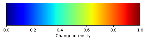
Areas with no changes are in blue tones; areas with significant changes are in red tones.

Input

Input of the DISMapper service consists of multiple Optical Calibrated Datasets derived from Sentinel-2 L2A images and two Auxiliary Datasets (Copernicus GLO30 DEM, ESA WorldCover). The service automatically retrieves all necessary Calibrated and Auxiliary Datasets in the Charter Mapper catalog. The user does not need to specify the input datasets.

S2 L2A ingestion scenario

Temporal coverage Once the activation workspace is created for a disaster activation and the AOIs are defined, the Charter Mapper ingests and calibrates the Sentinel-2 L2A images and prepares the inputs for DISMapper.

For the ingestion and calibration of Sentinel-2 L2A data, the following criteria are used:

Criteria	Pre-event image collection	Post-event image collection
Compulsory number of images	6	Depending on cloud coverage, until Charter activation.
Temporal Coverage	Search for 6 images acquired 45 days before the date of the disaster event. Else #1: Search for missing images in the period 395 to 335 days before the date of the disaster event. Else #2: Search for missing images in the period 335 to 30 days before the date of the disaster event.	All images acquired after the end of the disaster event.
Cloud coverage	<=75%	<=25%

Spatial coverage - only Sentinel-2 L2A images with footprints in the Charter activation AOIs.

Parameters

DISMapper requires mandatory and optional parameters listed in Table 1.

Parameter	Description	Required	Default value
Start date of the event	Starting date of the event in the format `YYYYMMDD`	YES
Search for post-event images after this date	Search for post-event images after this date in the format `YYYYMMDD` (e.g. when the event is ended)	NO	If empty, the service searches for post-event images acquired just after the start date of the event (e.g. assuming that the event is ended in 1 day)
Hazard event type	Select the hazard type among: `wildfire`, `landslide`, `flood` or `volcano`	YES
Area of Interest (AOI) in WKT	AOI in WKT format. The AOI intersects with the Sentinel-2 image footprints and the extent of the auxiliary datasets.	YES
Cloud coverage pre-event	Cloud coverage threshold applied to the pre event products selection (0-25)	YES
Cloud coverage post-event	Cloud coverage threshold applied to the post event products selection (0-75)	YES

Table 1 - DISMapper service parameters.

Disaster event dates

The user indicates the start and end dates of the disaster event in the form YYYYMMDD (e.g. 20230220). All the Sentinel-2 images acquired between these two dates will be queried but only those fulfilling the criteria will be ingested in the processing.

Area of interest in WKT

The geometry of the AOI is expressed in Well-Known Text file format (WKT). The activation AOIs is the extent of all auxiliary data available in the activation workspace and consists of a rectangular bounding box. If the AOI intersects more than one Sentinel-2 tile, the service takes the tile that has the greater intersection with the AOI.

Warning

The input area of interest must be contained within the activation AOIs envelope and contained with the footprint of a Sentinel-2 L2A image.

Tip

In the definition of “Area of interest as Well-Known Text”, it is possible to apply as AOI the polygon defined with the area filter. To do so, click on the button in the left side of the "Area of Interest expressed as Well-known text" box and select the option AOI from the list. The platform will automatically fill the parameter value with the rectangular bounding box taken from the current search area.

Output

DISMapper provides the following products:

NRDI_c (Normalized Relative Difference Index - continuous data values; 10 m spatial resolution raster)
NRDI_c overview
NRDI_t (Normalized Relative Difference Index - binary data values; 10 m spatial resolution raster)
NRDI_t overview
Pre-event image composite (RGB) overview (10 m spatial resolution raster)
Post-event image composite (RGB) overview (10 m spatial resolution raster)

DISMapper single image products specifications are described in the below tables.

NRDI continuous single band

Attribute	Value / description
Long Name	NRDI_c: Normalized Relative Difference Index - continuous data values (single band)
Short Name	DISMapper_NRDI_c
Description	Normalized Relative Difference Index from 0 to 1
Data Type	Float32
Band	1
Format	COG
Projection	UTM
Valid Range	[0 - 1]
Fill Value	N/A

NRDI continuous overview

Attribute	Value / description
Long Name	Normalized Relative Difference Index - continuous data values (RGB composite)
Short Name	Overview_DISMapper_NRDI_c
Description	Visual product derived from the NRDI_c product [0,1] using a "BlueYellowRed" color map. Areas with no change are in blue tones; areas with significant change are in red tones.
Data Type	Unsigned 8-bit Integer
Band	4
Format	COG
Projection	UTM
Valid Range	[1 - 255]
Fill Value	0

NRDI binary single band

Attribute	Value / description
Long Name	Normalized Relative Difference Index - binary data values (single band)
Short Name	DISMapper_NRDI_t
Description	Binary product derived from the binarization of the NRDI_c. 0=no change 1=change
Data Type	Unsigned 8-bit Integer
Band	1
Format	COG
Projection	UTM
Valid Range	[0,1]
Fill Value	N/A

NRDI binary overview

Attribute	Value / description
Long Name	NRDI_t: Normalized Relative Difference Index - binary data values (RGB composite)
Short Name	Overview_DISMapper_NRDI_t
Description	Visual product derived from the NRDI_t product with transparency. Pixels in red tones show detected change
Data Type	Unsigned 8-bit Integer
Band	4
Format	COG
Projection	UTM
Valid Range	[1 - 255]
Fill Value	0

RGB pre-event overview

Attribute	Value / description
Long Name	Pre-event image composite (RGB) composite
Short Name	Overview_DISMapper_rgb_composite_pre
Description	Visual product derived from the 3 visible bands of the greenest pixel image composite pre-event
Data Type	Unsigned 8-bit Integer
Band	4
Format	COG
Projection	UTM
Valid Range	[1 - 255]
Fill Value	0

RGB post-event overview

Attribute	Value / description
Long Name	Post-event image composite (RGB) composite
Short Name	Overview_DISMapper_rgb_composite_post
Description	Visual product derived from the 3 visible bands of the greenest pixel image composite post-event
Data Type	Unsigned 8-bit Integer
Band	4
Format	COG
Projection	UTM
Valid Range	[1 - 255]
Fill Value	0

Vectorize DISMapper change detection single band asset

The DISMapper NRDI_t product can be filtered spatially and/or converted to polygons using the FilterVectorize service.

To polygonize the NRDI_t, single band asset employs the FilterVectorize service in Vectorize mode by selecting the true values DN=1 (change).

The FilterVectorize service can be used to post-process the NRDI_t product and remove isolated pixels. Thus to obtain spatially filtered change extent vector, use the FilterVectorize service in the Filter and Vectorize mode.

Warning

Only the NRDI_t single band asset can be used with the FilterVectorize service.

Scheip, C. M. and Wegmann, K. W.: HazMapper: a global open-source natural hazard mapping application in Google Earth Engine, Nat. Hazards Earth Syst. Sci., 21, 1495–1511, https://doi.org/10.5194/nhess-21-1495-2021, 2021. ↩
Montero, D., Aybar, C., Mahecha, M.D. et al. A standardized catalogue of spectral indices to advance the use of remote sensing in Earth system research. Sci Data 10, 197 (2023). https://doi.org/10.1038/s41597-023-02096-0 ↩
Rouse J., Haas R. H., Schell J. A., Deering D. (1973), “Monitoring vegetation systems in the great plains with ERTS”, NASA. Goddard Space Flight Center 3d ERTS-1 Symp., Vol. 1, Sect. A. Available at: ntrs.nasa.gov ↩
Huete, A.R., 1988. A Soil-Adjusted Vegetation Index (SAVI). Remote Sens. 309, 295–309. https://doi.org/10.1016/0034-4257(88)90106-X ↩
Baret, F., Guyot, G., Major, D.J., 1989. TSAVI: A vegetation index which minimizes soil brightness effects on LAI and APAR estimation. Dig. - Int. Geosci. Remote Sens. Symp. 3, 1355–1358. https://doi.org/10.1109/igarss.1989.576128 ↩
Key, C. H. and Benson, N. C. (2006), “Landscape Assessment (LA): Sampling and Analysis Methods”, USDA Forest Service Gen Tech. Rep RMRS-GTR-164-CD. FIREMON Fire effects monitoring and inventory System. Available at: fs.fed.us. ↩
Escadafal, R., Girard, M.C., Courault, D., 1989. Munsell soil color and soil reflectance in the visible spectral bands of landsat MSS and TM data. Remote Sens. Environ. 27, 37–46. https://doi.org/10.1016/0034-4257(89)90035-7 ↩
Alcaras, E., Costantino, D., Guastaferro, F., Parente, C. & Pepe, M. Normalized Burn Ratio Plus (NBR+): A New Index for Sentinel-2 Imagery. Remote Sensing 14, 1727, https://doi.org/10.3390/RS14071727 (2022). ↩