IRIS service specifications

This service performs a Change Detection using a pair of calibrated optical single band assets from the same or different EO missions, or a pair of SAR single band assets acquired from the same sensor. The service supports also a pair of spectral index or coherence single band assets derived from the same mission with other on-demand processors. The output consists of multiple change detection products derived from the Structural Similarity Index that show intensity, extent, and contours of the detected changes in the region of interest.

The tutorial of the IRIS service is available in this section.

Service Description

The Change Detection Analysis (IRIS) is a processing service developed by NHAZCA S.r.l. that implements image-processing algorithms for the monitoring of ground and structural changes.

The Change Detection Analysis takes as input a pair of pre- and post-event single band assets (reflectance, backscatter, spectral index, coherence, etc.), as it calculates the changes occurring in the secondary image with respect to the reference image. If the input is SAR assets, they must come from the same EO mission; if they are optical assets, they can come from different EO missions.

It derives multiple change detection products derived from the Structural Similarity Index Measure (SSI or SSIM)¹ computed on the input pair of single band assets.

cover

Info

The service supports single-band assets from Optical or Radar Calibrated Datasets representing reflectance or Sigma Nought in dB. It also supports single band assets from Results of on demand processing with the following services: OPT-Index, BAS, SAR-COIN, or STACK.

Note

Pre- and post-event Reflectance single band assets can come from a pair of Optical Calibrated Dataset having different EO mission.

Warning

Pre- and post-event Sigma Nought single band assets must come from a pair of SAR Calibrated Dataset having the same EO mission.

Warning

When employing outputs of other on-demand processing in IRIS, pre- and post-event single band assets must come from a pair of OPT-Index, BAS, SAR-COIN or STACK Results derived from the same EO mission.

IRIS pre-processing

Starting from the reading of the input pair of single band assets, IRIS first employs a Spatial Subset and resampling based on the AOI defined by the user.

The processor will automatically crop the images on the maximum common area and, if needed, resample one of the two images to match the Ground Sample Distance (GSD) of the other.

An optional co-registration step can then be applied to ensure the alignment of the two images with as much precision as possible, this is achieved employing a full field displacement measurement based on the Dense Inverse Search method for Optical Flow², which results are used to align the secondary image minimizing the residual shift.

If needed a binary mask (e.g. a cloud mask derived by another processor) can be also imported by the user to mask the pair co-located or co-registered single band assets.

IRIS change detection algorithm

After image normalization, the change detection algorithm is triggered to produce a Structural Similarity Index Measure (SSI or SSIM) map¹, that graphically and numerically displays the occurred changes. The Structural Similarity Index is defined as:

\[ SSIM(x,y) = \frac {(2 μ_x μ_y + C_1) \times (2 σ_{xy} + C_2)} {(μ^2_x + μ^2_y + C_1) \times (σ^2_x + σ^2_y + C_2)} \]

where: \(μ_x\) (\(μ_y\)), \(σ_x\) (\(σ_y\)) and \(σ_{xy}\) are, respectively, the average (weighted with a Gaussian filter), standard deviation and cross-covariance for x (y) image patch, C1 and C2 are variables which depends on the dynamic range of the pixels.

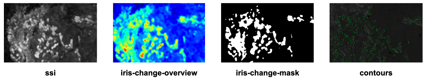
The SSI is computed on a sliding window (patch) of fixed size and the value is assigned to the central pixel of the window. The results consist of numerical map (ssi single band asset) with a value in the range [0 – 1] assigned to each pixel of the region of interest, where 1 is the maximum SSI (representing a perfect similarity between images) and 0 is the minimum SSIM value (representing the maximum observable change).

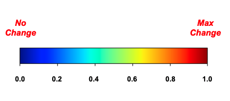
To create the SSI overview product, the change maps are then converted in a coloured overlay map which can be superimposed to the original image to create an easily and immediately understandable product in a range of 0 (no changes) – 1 (maximum change). The images obtained in this way are three-band geotiff with transparency (RGBA) that can be imported in any GIS environment (overview-iris multi-band asset). The multicolor color map adopted in the creation of the RGBA is the following:

Legend-001

The processor makes a binarization of the SSI asset using a threshold value, between 0 and 1, defined by the user to obtain the IRIS binary change mask. The obtained binary mask (iris-change-mask single band asset) is then used by the processor for the detected change contouring and creating the Contours overview product, which is a RGBA with the pre-event single band asset in gray scale and superimposed contours in yellow (contours multi-band asset).

IRIS post-processing

In the final step of the IRIS processing a water masking of the 4 change detection products (ssi, overview-iris, iris-change-mask, and contours assets) is done by using the Global Surface Water 1984-2020 Transitions auxiliary data³,⁴. The permanent water mask is derived from the GSW Transitions dataset using classes: Permanent, New Permanent, and Seasonal to Permanent.

Info

By default IRIS produces in output the 4 change detection products not masked by water (ssi, overview-iris, iris-change-mask, and contours) and a copy of them in which permanent waters are masked out (ssi-no-water, overview-iris-no-water, iris-change-mask-no-water, and contours-no-water).

Note

The mask of permanent waters employed in the IRIS post-processing is not part of the service output.

Workflow

The IRIS service implements the workflow depicted below.

graph TB c[(Datasets, Aux Datasets <br> or Results)] style c fill:#ffde86,stroke:#333,color:#282828,stroke-width:2px c --> b1(Pre-event Dataset or Result) c --> b2(Pre-event Dataset or Result) b2 --> a2[input 2] b1 --> a1[input 1] subgraph Inputs style Inputs fill:#e8e8e8,stroke:#818181,color:#282828 a1[/Reference asset/] style a1 fill:#acc8ff,stroke:#333,color:#282828,stroke-width:2px a2[/Secondary asset/] style a2 fill:#acc8ff,stroke:#333,color:#282828,stroke-width:2px a3[/AOI as WKT/] style a3 fill:#acc8ff,stroke:#333,color:#282828,stroke-width:2px a4[/Window size/] style a4 fill:#acc8ff,stroke:#333,color:#282828,stroke-width:2px a5[/Threshold/] style a5 fill:#acc8ff,stroke:#333,color:#282828,stroke-width:2px a6[/Binary mask/] style a6 fill:#acc8ff,stroke:#333,color:#282828,stroke-width:2px end subgraph IRIS a1 --> ssar[Spatial subset and resampling] a2 --> ssar[Spatial subset and resampling] a3 -.-> ssar[Spatial subset and resampling] ssar --> coreg[Co-registration] coreg --> p1(Reference asset) style p1 fill:#cfdfff,stroke:#333,color:#282828 coreg --> p2(Secondary asset) style p2 fill:#cfdfff,stroke:#333,color:#282828 coreg --> norm[Images normalization] a3 -.-> cda[Change detection algorithm] a4 --> cda[Change detection algorithm] norm --> cda[Change detection algorithm] cda --> p3(ssi) style p3 fill:#cfdfff,stroke:#333,color:#282828 p3 --> over[SSI Overview and legend creation] p3 --> bin[SSI Binarization] a5 --> bin[SSI Binarization] bin --> p5(binary) style p5 fill:#cfdfff,stroke:#333,color:#282828 bin --> over2[Contours Overview creation] over2 --> p6(contours) style p6 fill:#cfdfff,stroke:#333,color:#282828 over --> p4(overview-iris) style p4 fill:#cfdfff,stroke:#333,color:#282828 p1 --> cog[Convert to COG] p2 --> cog[Convert to COG] a6 -.-> binmas[Binary Masking] binmas -.-> watmas[Water Masking] p3 --> watmas[Water Masking] p4 --> watmas[Water Masking] p5 --> watmas[Water Masking] p6 --> watmas[Water Masking] watmas --> cog[Convert to COG] cog --> stac[Create STAC item] end subgraph Outputs style Outputs fill:#e8e8e8,stroke:#818181,color:#282828 stac --> o1[/Reference asset/] style o1 fill:#acc8ff,stroke:#87afff,color:#282828,stroke-width:2px stac --> o2[/Secondary co-registered asset/] style o2 fill:#acc8ff,stroke:#87afff,color:#282828,stroke-width:2px stac --> o3[/SSI index/] style o3 fill:#acc8ff,stroke:#87afff,color:#282828,stroke-width:2px stac --> o4[/IRIS overview/] style o4 fill:#acc8ff,stroke:#87afff,color:#282828,stroke-width:2px stac --> o5[/Binary map from SSI/] style o5 fill:#acc8ff,stroke:#87afff,color:#282828,stroke-width:2px stac --> o6[/Contours/] style o6 fill:#acc8ff,stroke:#87afff,color:#282828,stroke-width:2px end

Inputs

Input of the IRIS service is a couple of single band reflectance (or backscatter) assets from two Calibrated Datasets [CD] or a pair of single band assets from two Results of OPT-Index, BAS, SAR-COIN or STACK services:

a pre-event single band asset (reflectance, backscatter, spectral index, or coherence),
and a post-event single band asset (reflectance, backscatter, spectral index, or coherence).

Note

Pre- and post-event Reflectance single band assets can come from a pair of Optical Calibrated Dataset having different EO mission. As an example, a pair of red single band assets from a Worldview-2 (pre-event) and WorldView-3 (post-event) Calibrated Datasets.

Warning

Pre- and post-event Sigma Nought single band assets must come from a pair of SAR Calibrated Dataset having the same EO mission. As an example, a pair of s0_db_c_vv single band assets from two Sentinel-1 GRD (pre- and post-event) Calibrated Datasets.

Warning

The pair of input single band assets shall have the same CBN (e.g. red for both pre- and post-event calibrated single band assets).

Warning

When employing outputs of other on-demand processing in IRIS, pre- and post-event single band assets must come from a pair of OPT-Index, BAS, SAR-COIN or STACK Results derived from the same EO mission. As an example, a pair of ndvi single band assets from two OPT-Index Results (pre- and post-event) derived from two Sentinel-2 Calibrated Datasets.

Note

To get better results from the Change Detection Analysis service it is better to use a co-registered pair of single band assets having the same GSD.

Parameters

The IRIS service requires mandatory and optional parameters. All service parameters are listed in the below Table 1.

Parameter	Description	Required	Default value
Pre-event single band asset	Product reference to reference single band asset used in the change detection analysis	YES
Post-event single band asset	Product reference to secondary single band asset used in the change detection analysis	YES
Optional mask	Product reference to single band binary asset to mask iris change detection results	NO
Window size	Extension of the sliding window used to perform the change detection	YES	41
Threshold	A threshold value, between 0 and 1, for the detected change contouring	YES	0.4
Co-registration method	A flag to employ `Rigid` or `Elastic` co-regitration of input assets. `None` to not perform the co-registration.	YES	Rigid
Area of Interest	A polygon representing the area of interest to be analysed in WKT format	NO

Table 1 - Service parameters for the IRIS processor.

Pre and post event single band asset

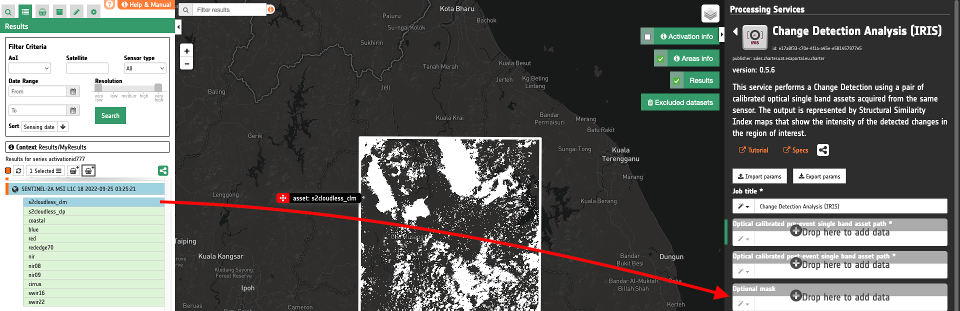
The first two mandatory parameters define the input "Reference" and "Secondary" images from Optical or SAR Calibrated Datasets or Results from OPT-Index, BAS, SAR-COIN or STACK services. Input for Pre-event single band asset and Post-event single band asset parameters are the path to the single band assets from the two Calibrated Datasets or Results STAC items. This parameter is required to specify both the reference to the Calibrated Dataset and the STAC key of the single band asset (specified as CBN for calibrated Datasets or asset name for Results) to use for the analysis (e.g. red, s0_db_c_vv, ndvi, etc).

In the definition of the input single band asset the drag and drop of the single-band asset is foreseen. This is possible by dragging and dropping one of the single-band assets (CBNs) included into a Calibrated Dataset retrieved from the features in the Results panel or in the feature basket.

Hint

To consult the bands of a Calibrated Dataset, click on the Show assets button available near the feature title. A list with all single-band assets (CBNs) included within the Calibrated Dataset will appear under the feature title.

Image-note-001

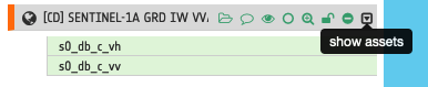
Same to find single band assets from Results of on-demand processing.

The drag and drop of the single band asset provides to the service the reference to the input calibrated dataset in the format

input_dataset_reference#single-band_asset

Note

This string format is the only type of input accepted.

As an example, after the drag and drop of a feature the following string will be automatically inserted as a value for the parameter:

https://catalog.disasterscharter.org//charter/cat/[chartercalibrateddataset,{callid895}]/search?format=json&uid=call895_PT01N07_966794E007_8043502022080500000000MS00_GG003002001-calibrated#nir"

Warning

Users must drag and drop the single-band asset (e.g. nir for reflectance or s0_db_c_vv for backscatter in VV polarization and C-band) into both Pre-event single band asset and Post-event single band asset fields. The drag and drop of the Calibrated Dataset (e.g. "[CD] PLANETSCOPE PSB.SD L3B 2022-08-05 09:01:35") is not enough.

Optional mask

In this optional parameter the user can insert a binary single band asset (e.g. a cloud mask from the S2-Cloudless) contained within a Dataset or into a Result feature derived from another service. If specified, this asset will be used to mask iris change detection results.

Optional mask figure

Tip

To fill the parameter just drag and drop the single band asset (e.g. the s2cloudless_clm single band asset from a Result of S2-Cloudless).

Window size

The user must provide a value for the window size, which defines the size of the sliding window in pixels, this parameter can highly influence the result of the analysis. The higher this parameter is set, the more averaged the change map will be, while the smaller and the more detailed changes can be identified at the cost of potentially noisier results. This is due to the SSIM value for each pixel being computed using the information present in the whole sliding window, thus obtaining a more localized value of the index in case of a smaller window. As a rule of thumb, the dimension of the window should be set in a range between 9 and 71. This range depends on the type of changes the user wants to identify. The output SSIM maps will have the same Ground Sample Distance of the selected band.

Warning

Window size shall be in a range between 9 and 71. The inserted value must be odd.

Note

Default value is 41.

Threshold

In this mandatory parameter the user shall provide a value between 0 and 1 to be used for the binarization of SSI and detected change contouring.

Co-registration method

In this mandatory parameter the service offers the possibility to co-register the secondary single band asset to the reference one. The user can choose among an Elastic or a Rigid co-registration of input assets. In case the co-registration is not needed, the processor does a co-location of input assets over a common grid.

The co-registration parameter can be set to one of the following values:

None the co-registration is not performed,
Rigid the full-field displacement measured is used to estimate an Affine transformation matrix which is then applied to the secondary image,
Elastic the full-field displacement is used to freely warp the secondary image.

Note

Default value is Rigid.

AOI (optional)

This last parameter (optional) may define the area of interest expressed as a Well-Known Text value.

Tip

In the definition of “Area of interest as Well Known Text” it is possible to apply as AOI the drawn polygon defined with the area filter. To do so, click on the button in the left side of the "Area of interest expressed as Well-known text" box and select the option AOI from the list. The platform will automatically fill the parameter value with the rectangular bounding box taken from the current search area in WKT format.

Output

The IRIS processor provides as output the following products:

The co-located or co-registered pair of input single-band assets,
SSI index (ssi single band asset),
SSI change detection overview (overview-iris multi band asset),
Binary mask from thresholding of SSI (iris-change-mask single band asset),
Detected change contours overview (contours multi band asset).

The first output product is the co-located or co-registered pair of single-band assets derived within the IRIS processing.

Warning

Output single band pre- and post-event assets are not the original rasters from Calibrated Datasets or Results but are altered by the warping and co-registration in IRIS.

The second one is a georeferenced single band image containing the value of the SSIM assigned to each pixel of the region of interest with values between 0 (maximum observable change) and 1 (perfect similarity between images).

The third one represents a georeferenced RGB representation of the SSIM map with an associated colorbar legend. The forth product is a binary map derived from the SSI index using the user defined threshold.

Warning

The output binary change mask iris-change-mask derived from thresholding of SSI has the following pixel values: Change = 255 and No-Change = 0.

The last product is a RGBA with the pre-event single band asset in gray scale and superimposed detected change contours in yellow.

After the masking of permanent waters from products 2, 3, 4, and 5, IRIS also gives in output:

SSI index with masking of permanent waters (ssi-no-water single band asset),
SSI change detection overview with masking of permanent waters (overview-iris-no-water multi band asset),
Binary mask from thresholding of SSI with masking of permanent waters (iris-change-mask-no-water single band asset),
Detected change contours overview with masking of permanent waters (contours-no-water multi band asset).

IRIS Product Specifications can be found in the below tables.

Co-registered input single band asset

Attribute	Value / description
Long Name	Co-located or Co-registered single band assets
Short Name	asset_pre, asset_post (e.g. `nir_pre` and `nir_post` or `s0_db_c_vv_pre` and `s0_db_c_vv_post`, `ndvi_pre` and ndvi_post`)
Description	Co-registered pair from input single band assets (reflectance, backscatter, spectral index or coherence)
Data Type	As per the input images (e.g. UInt16 for reflectance)
Band	1
Format	COG
Projection	As per input single band asset
Valid Range	As per input single band asset
Fill Value	As per input single band asset

SSIM values

Attribute	Value / description
Long Name	SSI index
Short Name	ssi, ssi-no-water
Description	SSIM value assigned to every pixel of the image with/without masking of permanent waters
Data Type	Float 32
Band	1
Format	COG
Projection	As per the input images (UInt16 for reflectance assets)
Valid Range	[0 - 1]
Fill Value	NaN

SSI overview

Attribute	Value / description
Long Name	SSI change detection overview
Short Name	overview-iris, overview-iris-no-water
Description	RGBA colour composite representing the SSIM map with/without masking of permanent waters
Data Type	Unsigned 8-bit Integer
Band	4
Format	COG
Projection	As per the input images
Valid Range	[1 - 255]

Binary map

Attribute	Value / description
Long Name	Binary map from SSI
Short Name	iris-change-mask, iris-change-mask-no-water
Description	Binary change mask derived from thresholding of SSI True=`255` False=`0` with/without masking of permanent waters
Data Type	Unsigned 8-bit Integer
Band	1
Format	COG
Projection	As per the input images
Valid Range	[0,255]
Fill Value	0

Contours overview

Attribute	Value / description
Long Name	Detected change contours overview
Short Name	contours, contours-no-water
Description	RGBA showing the pre-event single band asset in gray scale and superimposed detected change contours in yellow with/without masking of permanent waters
Data Type	Unsigned 8-bit Integer
Band	4
Format	COG
Projection	As per the input images
Valid Range	[1 - 255]

Filter and or Vectorize IRIS binary single band asset

IRIS's binary change asset can be spatially filtered and / or converted to polygon using the FilterVectorize service.

To further post-process the iris-change-mask single band asset by removing small isolated clusters of pixel employ the FilterVectorize service in Filter mode by selecting a filter threshold size value.

The binary change mask can also be converted to polygons by using the FilterVectorize service in Vectorize mode and selecting only true values DN=255 (change).

To apply both spatial filtering and vectorization on IRIS's binary change mask employ the FilterVectorize service in the Filter and Vectorize mode.

Warning

Only the iris-change-mask single band asset can be used in the FilterVectorize on-demand service, being the only discrete raster produced by the IRIS service.

Zhou, W., A. C. Bovik, H. R. Sheikh, and E. P. Simoncelli, (2004) "Image Quality Assessment: From Error Visibility to Structural Similarity." IEEE Transactions on Image Processing. Vol. 13, Issue 4, April 2004, pp. 600–612. DOI: 10.1109/TIP.2003.819861. ↩↩
Kroeger, T., Timofte, R., Dai, D., Van Gool, L. (2016), "Fast Optical Flow Using Dense Inverse Search", In: Leibe, B., Matas, J., Sebe, N., Welling, M. (eds) Computer Vision – ECCV 2016. Lecture Notes in Computer Science, vol 9908. Springer, Cham. DOI: 10.1007/978-3-319-46493-0_29. ↩
Pekel, JF., Cottam, A., Gorelick, N. et al. High-resolution mapping of global surface water and its long-term changes. Nature 540, 418–422 (2016). DOI: 10.1038/nature20584. ↩
Global Surface Water 1984-2020, Occurrence, Occurrence change intensity, Seasonality, Recurrence, Transitions, and Maximum water extent. More info at: global-surface-water.appspot.com. ↩